

Chapter 62
Properties of Laplace
transforms
62.1 The Laplace transform of e
at f (t)
From Chapter 61, the definition of the Laplace transform
of f (t ) is:
L{ f (t )} =
∞
0
e
−st f (t ) dt
(1)
Thus L{e
at f (t )} =
∞
0
e
−st
(e
at f (t )) dt
=
∞
0
e
−(s−a) f (t ) dt
(2)
(where a is a real constant)
Hence the substitution of (s − a) for s in the transform
shown in equation (1) corresponds to the multiplication
of the original function f (t ) by e at . This is known as a
shift theorem.
62.2 Laplace transforms of the form
e at f(t)
From equation (2), Laplace transforms of the form
e at f (t ) may be deduced. For example:
(i) L{e at t n }
Since L{t n } =
n!
s n+1 from (viii) of Table 61.1,
page 584.
then L{e at t n } =
n!
(s − a)
n+1
from equation (2)
above (provided s > a).
(ii) L{e at sin ωt}
Since L{sin ωt } =
ω
s 2 + ω 2 from (iv) of Table
61.1, page 584.
then L{e at sin ωt} =
ω
(s −a)
2
+ ω 2
from equation (2) (provided s > a).
(iii) L{e
at cosh ωt}
Since L{cosh ωt } =
s
s 2 − ω 2 from (ix) of Table
61.1, page 584.
then L{e at cosh ωt} =
s − a
(s − a) 2 − ω 2
from equation (2) (provided s > a).
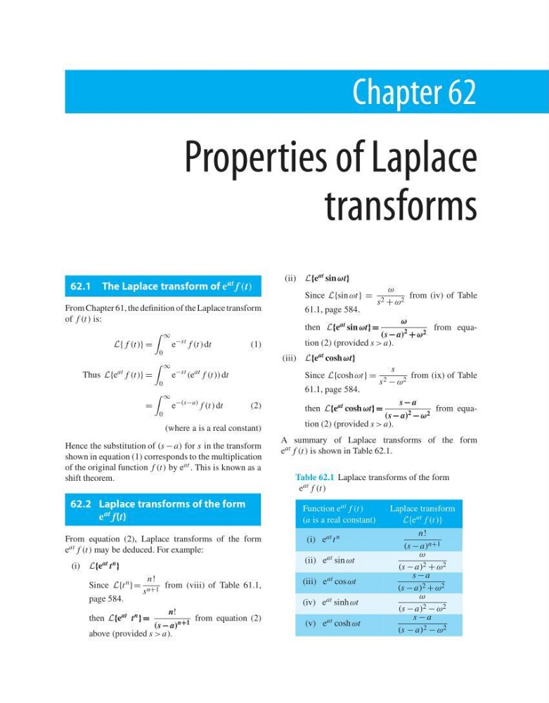
A summary of Laplace transforms of the form
e at f (t ) is shown in Table 62.1.
Table 62.1 Laplace transforms of the form
e at f (t )
Function e at f (t )
Laplace transform
(a is a real constant)
L{e at f (t )}
(i) e at t n
n!
(s − a) n+1
(ii) e at sin ωt
ω
(s − a) 2 + ω 2
(iii) e at cos ωt
s − a
(s − a) 2 + ω 2
(iv) e at sinh ωt
ω
(s − a) 2 − ω 2
(v) e at cosh ωt
s − a
(s − a) 2 − ω 2
Properties of Laplace
transforms
62.1 The Laplace transform of e
at f (t)
From Chapter 61, the definition of the Laplace transform
of f (t ) is:
L{ f (t )} =
∞
0
e
−st f (t ) dt
(1)
Thus L{e
at f (t )} =
∞
0
e
−st
(e
at f (t )) dt
=
∞
0
e
−(s−a) f (t ) dt
(2)
(where a is a real constant)
Hence the substitution of (s − a) for s in the transform
shown in equation (1) corresponds to the multiplication
of the original function f (t ) by e at . This is known as a
shift theorem.
62.2 Laplace transforms of the form
e at f(t)
From equation (2), Laplace transforms of the form
e at f (t ) may be deduced. For example:
(i) L{e at t n }
Since L{t n } =
n!
s n+1 from (viii) of Table 61.1,
page 584.
then L{e at t n } =
n!
(s − a)
n+1
from equation (2)
above (provided s > a).
(ii) L{e at sin ωt}
Since L{sin ωt } =
ω
s 2 + ω 2 from (iv) of Table
61.1, page 584.
then L{e at sin ωt} =
ω
(s −a)
2
+ ω 2
from equation (2) (provided s > a).
(iii) L{e
at cosh ωt}
Since L{cosh ωt } =
s
s 2 − ω 2 from (ix) of Table
61.1, page 584.
then L{e at cosh ωt} =
s − a
(s − a) 2 − ω 2
from equation (2) (provided s > a).
A summary of Laplace transforms of the form
e at f (t ) is shown in Table 62.1.
Table 62.1 Laplace transforms of the form
e at f (t )
Function e at f (t )
Laplace transform
(a is a real constant)
L{e at f (t )}
(i) e at t n
n!
(s − a) n+1
(ii) e at sin ωt
ω
(s − a) 2 + ω 2
(iii) e at cos ωt
s − a
(s − a) 2 + ω 2
(iv) e at sinh ωt
ω
(s − a) 2 − ω 2
(v) e at cosh ωt
s − a
(s − a) 2 − ω 2