

468 Higher Engineering Mathematics
y C 1 = y 0 +
1
2 h[(y
) 0 + f (x 1 , y P 1 )]
= 2.89090205 +
1
2 (0.1)[2.49090205
+ (3.139992255 − 0.5)]
= 3.147446765
Problem 4 is the same example as Problem 3 and
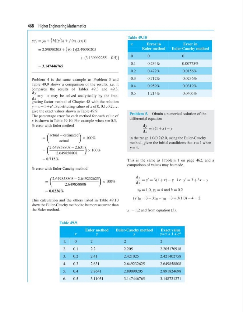
Table 49.9 shows a comparison of the results, i.e. it
compares the results of Tables 49.3 and 49.8.
d y
dx
= y − x may be solved analytically by the integrating factor method of Chapter 48 with the solution
y = x + 1 +e x . Substituting values of x of 0, 0.1, 0.2, ...
give the exact values shown in Table 49.9.
The percentage error for each method for each value of
x is shown in Table 49.10. For example when x = 0.3,
% error with Euler method
=
actual − estimated
actual
× 100%
=
2.649858808 − 2.631
2.649858808
× 100%
= 0.712%
% error with Euler-Cauchy method
=
2.649858808 − 2.649232625
2.649858808
× 100%
= 0.0236%
This calculation and the others listed in Table 49.10
show the Euler-Cauchy method to be more accurate than
the Euler method.
Table 49.10
x
Error in
Error in
Euler method
Euler-Cauchy method
0
0
0
0.1
0.234%
0.00775%
0.2
0.472%
0.0156%
0.3
0.712%
0.0236%
0.4
0.959%
0.0319%
0.5
1.214%
0.0405%
Problem 5. Obtain a numerical solution of the
differential equation
d y
dx
= 3(1 + x) − y
in the range 1.0(0.2)2.0, using the Euler-Cauchy
method, given the initial conditions that x = 1 when
y = 4.
This is the same as Problem 1 on page 462, and a
comparison of values may be made.
d y
dx
= y
= 3(1 + x) − y i.e. y
= 3 + 3x − y
x 0 = 1.0, y 0 = 4 and h = 0.2
(y
) 0 = 3 + 3x 0 − y 0 = 3 + 3(1.0) − 4 = 2
x 1 = 1.2 and from equation (3),
Table 49.9
Euler method
Euler-Cauchy method
Exact value
x
y
y
y = x+1 + e
x
1.
0
2
2
2
2.
0.1
2.2
2.205
2.205170918
3.
0.2
2.41
2.421025
2.421402758
4.
0.3
2.631
2.649232625
2.649858808
5.
0.4
2.8641
2.89090205
2.891824698
6.
0.5
3.11051
3.147446765
3.148721271
y C 1 = y 0 +
1
2 h[(y
) 0 + f (x 1 , y P 1 )]
= 2.89090205 +
1
2 (0.1)[2.49090205
+ (3.139992255 − 0.5)]
= 3.147446765
Problem 4 is the same example as Problem 3 and
Table 49.9 shows a comparison of the results, i.e. it
compares the results of Tables 49.3 and 49.8.
d y
dx
= y − x may be solved analytically by the integrating factor method of Chapter 48 with the solution
y = x + 1 +e x . Substituting values of x of 0, 0.1, 0.2, ...
give the exact values shown in Table 49.9.
The percentage error for each method for each value of
x is shown in Table 49.10. For example when x = 0.3,
% error with Euler method
=
actual − estimated
actual
× 100%
=
2.649858808 − 2.631
2.649858808
× 100%
= 0.712%
% error with Euler-Cauchy method
=
2.649858808 − 2.649232625
2.649858808
× 100%
= 0.0236%
This calculation and the others listed in Table 49.10
show the Euler-Cauchy method to be more accurate than
the Euler method.
Table 49.10
x
Error in
Error in
Euler method
Euler-Cauchy method
0
0
0
0.1
0.234%
0.00775%
0.2
0.472%
0.0156%
0.3
0.712%
0.0236%
0.4
0.959%
0.0319%
0.5
1.214%
0.0405%
Problem 5. Obtain a numerical solution of the
differential equation
d y
dx
= 3(1 + x) − y
in the range 1.0(0.2)2.0, using the Euler-Cauchy
method, given the initial conditions that x = 1 when
y = 4.
This is the same as Problem 1 on page 462, and a
comparison of values may be made.
d y
dx
= y
= 3(1 + x) − y i.e. y
= 3 + 3x − y
x 0 = 1.0, y 0 = 4 and h = 0.2
(y
) 0 = 3 + 3x 0 − y 0 = 3 + 3(1.0) − 4 = 2
x 1 = 1.2 and from equation (3),
Table 49.9
Euler method
Euler-Cauchy method
Exact value
x
y
y
y = x+1 + e
x
1.
0
2
2
2
2.
0.1
2.2
2.205
2.205170918
3.
0.2
2.41
2.421025
2.421402758
4.
0.3
2.631
2.649232625
2.649858808
5.
0.4
2.8641
2.89090205
2.891824698
6.
0.5
3.11051
3.147446765
3.148721271