

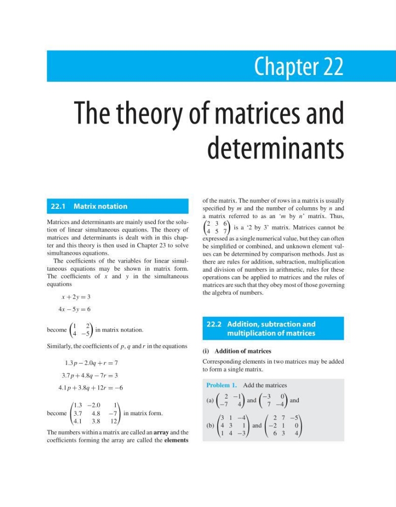
Chapter 22
The theory of matrices and
determinants
22.1 Matrix notation
Matrices and determinants are mainly used for the solution of linear simultaneous equations. The theory of
matrices and determinants is dealt with in this chapter and this theory is then used in Chapter 23 to solve
simultaneous equations.
The coefficients of the variables for linear simultaneous equations may be shown in matrix form.
The coefficients of x and y in the simultaneous
equations
x + 2y = 3
4x − 5y = 6
become
1
2
4 −5
in matrix notation.
Similarly, the coefficients of p, q and r in the equations
1.3 p − 2.0q + r = 7
3.7 p + 4.8q − 7r = 3
4.1 p + 3.8q + 12r = −6
become
⎛
⎝
1.3 −2.0
1
3.7
4.8 −7
4.1
3.8
12
⎞
⎠ in matrix form.
The numbers within a matrix are called an array and the
coefficients forming the array are called the elements
of the matrix. The number of rows in a matrix is usually
specified by m and the number of columns by n and
a matrix referred to as an ‘m by n’ matrix. Thus,
2 3 6
4 5 7
is a ‘2 by 3’ matrix. Matrices cannot be
expressed as a single numerical value, but they can often
be simplified or combined, and unknown element values can be determined by comparison methods. Just as
there are rules for addition, subtraction, multiplication
and division of numbers in arithmetic, rules for these
operations can be applied to matrices and the rules of
matrices are such that they obey most of those governing
the algebra of numbers.
22.2 Addition, subtraction and
multiplication of matrices
(i) Addition of matrices
Corresponding elements in two matrices may be added
to form a single matrix.
Problem 1. Add the matrices
(a)
2 −1
−7
4
and
−3
0
7 −4
and
(b)
⎛
⎝
3 1 −4
4 3
1
1 4 −3
⎞
⎠ and
⎛
⎝
2 7 −5
−2 1
0
6 3
4
⎞
⎠
The theory of matrices and
determinants
22.1 Matrix notation
Matrices and determinants are mainly used for the solution of linear simultaneous equations. The theory of
matrices and determinants is dealt with in this chapter and this theory is then used in Chapter 23 to solve
simultaneous equations.
The coefficients of the variables for linear simultaneous equations may be shown in matrix form.
The coefficients of x and y in the simultaneous
equations
x + 2y = 3
4x − 5y = 6
become
1
2
4 −5
in matrix notation.
Similarly, the coefficients of p, q and r in the equations
1.3 p − 2.0q + r = 7
3.7 p + 4.8q − 7r = 3
4.1 p + 3.8q + 12r = −6
become
⎛
⎝
1.3 −2.0
1
3.7
4.8 −7
4.1
3.8
12
⎞
⎠ in matrix form.
The numbers within a matrix are called an array and the
coefficients forming the array are called the elements
of the matrix. The number of rows in a matrix is usually
specified by m and the number of columns by n and
a matrix referred to as an ‘m by n’ matrix. Thus,
2 3 6
4 5 7
is a ‘2 by 3’ matrix. Matrices cannot be
expressed as a single numerical value, but they can often
be simplified or combined, and unknown element values can be determined by comparison methods. Just as
there are rules for addition, subtraction, multiplication
and division of numbers in arithmetic, rules for these
operations can be applied to matrices and the rules of
matrices are such that they obey most of those governing
the algebra of numbers.
22.2 Addition, subtraction and
multiplication of matrices
(i) Addition of matrices
Corresponding elements in two matrices may be added
to form a single matrix.
Problem 1. Add the matrices
(a)
2 −1
−7
4
and
−3
0
7 −4
and
(b)
⎛
⎝
3 1 −4
4 3
1
1 4 −3
⎞
⎠ and
⎛
⎝
2 7 −5
−2 1
0
6 3
4
⎞
⎠