

Solving equations by iterative methods 81
f(x)
2
1
0
1
2
3
4
x
f(x)ϭϪxϩ2
f(x)ϭ 2In x
Ϫ1
Ϫ2
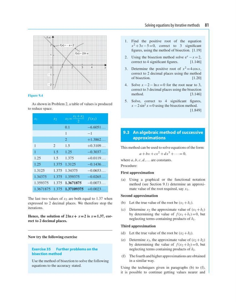
Figure 9.4
As shown in Problem 2, a table of values is produced
to reduce space.
x 1
x 2
x 3 =
x 1 + x 2
2
f (x 3 )
0.1
−6.6051 ...
1
−1
2
+1.3862 ...
1
2
1.5
+0.3109 ...
1
1.5
1.25
−0.3037 ...
1.25
1.5
1.375
+0.0119 ...
1.25
1.375 1.3125
−0.1436 ...
1.3125
1.375 1.34375
−0.0653 ...
1.34375
1.375 1.359375
−0.0265 ...
1.359375 1.375 1.3671875
−0.0073 ...
1.3671875 1.375 1.37109375 +0.0023 ...
The last two values of x 3 are both equal to 1.37 when
expressed to 2 decimal places. We therefore stop the
iterations.
Hence, the solution of 2 ln x + x = 2 is x = 1.37, correct to 2 decimal places.
Now try the following exercise
Exercise 35 Further problems on the
bisection method
Use the method of bisection to solve the following
equations to the accuracy stated.
1. Find the positive root of the equation
x
2
+ 3x − 5 = 0, correct to 3 significant
figures, using the method of bisection. [1.19]
2. Using the bisection method solve e x − x = 2,
correct to 4 significant figures.
[1.146]
3. Determine the positive root of x 2 = 4 cos x,
correct to 2 decimal places using the method
of bisection.
[1.20]
4. Solve x − 2 − ln x = 0 for the root near to 3,
correct to 3 decimal places using the bisection
method.
[3.146]
5. Solve, correct to 4 significant figures,
x − 2 sin 2 x = 0 using the bisection method.
[1.849]
9.3 An algebraic method of successive
approximations
This method can be used to solve equations of the form:
a + bx + cx
2
+ dx
3
+ · · · = 0,
where a, b, c, d, ... are constants.
Procedure:
First approximation
(a) Using a graphical or the functional notation
method (see Section 9.1) determine an approximate value of the root required, say x 1 .
Second approximation
(b) Let the true value of the root be (x 1 + δ 1 ).
(c) Determine x 2 the approximate value of (x 1 + δ 1 )
by determining the value of f (x 1 + δ 1 ) = 0, but
neglecting terms containing products of δ 1 .
Third approximation
(d) Let the true value of the root be (x 2 + δ 2 ).
(e) Determine x 3 , the approximate value of (x 2 + δ 2 )
by determining the value of f (x 2 + δ 2 ) = 0, but
neglecting terms containing products of δ 2 .
(f) The fourth and higher approximations are obtained
in a similar way.
Using the techniques given in paragraphs (b) to (f),
it is possible to continue getting values nearer and
f(x)
2
1
0
1
2
3
4
x
f(x)ϭϪxϩ2
f(x)ϭ 2In x
Ϫ1
Ϫ2
Figure 9.4
As shown in Problem 2, a table of values is produced
to reduce space.
x 1
x 2
x 3 =
x 1 + x 2
2
f (x 3 )
0.1
−6.6051 ...
1
−1
2
+1.3862 ...
1
2
1.5
+0.3109 ...
1
1.5
1.25
−0.3037 ...
1.25
1.5
1.375
+0.0119 ...
1.25
1.375 1.3125
−0.1436 ...
1.3125
1.375 1.34375
−0.0653 ...
1.34375
1.375 1.359375
−0.0265 ...
1.359375 1.375 1.3671875
−0.0073 ...
1.3671875 1.375 1.37109375 +0.0023 ...
The last two values of x 3 are both equal to 1.37 when
expressed to 2 decimal places. We therefore stop the
iterations.
Hence, the solution of 2 ln x + x = 2 is x = 1.37, correct to 2 decimal places.
Now try the following exercise
Exercise 35 Further problems on the
bisection method
Use the method of bisection to solve the following
equations to the accuracy stated.
1. Find the positive root of the equation
x
2
+ 3x − 5 = 0, correct to 3 significant
figures, using the method of bisection. [1.19]
2. Using the bisection method solve e x − x = 2,
correct to 4 significant figures.
[1.146]
3. Determine the positive root of x 2 = 4 cos x,
correct to 2 decimal places using the method
of bisection.
[1.20]
4. Solve x − 2 − ln x = 0 for the root near to 3,
correct to 3 decimal places using the bisection
method.
[3.146]
5. Solve, correct to 4 significant figures,
x − 2 sin 2 x = 0 using the bisection method.
[1.849]
9.3 An algebraic method of successive
approximations
This method can be used to solve equations of the form:
a + bx + cx
2
+ dx
3
+ · · · = 0,
where a, b, c, d, ... are constants.
Procedure:
First approximation
(a) Using a graphical or the functional notation
method (see Section 9.1) determine an approximate value of the root required, say x 1 .
Second approximation
(b) Let the true value of the root be (x 1 + δ 1 ).
(c) Determine x 2 the approximate value of (x 1 + δ 1 )
by determining the value of f (x 1 + δ 1 ) = 0, but
neglecting terms containing products of δ 1 .
Third approximation
(d) Let the true value of the root be (x 2 + δ 2 ).
(e) Determine x 3 , the approximate value of (x 2 + δ 2 )
by determining the value of f (x 2 + δ 2 ) = 0, but
neglecting terms containing products of δ 2 .
(f) The fourth and higher approximations are obtained
in a similar way.
Using the techniques given in paragraphs (b) to (f),
it is possible to continue getting values nearer and