Section 9.4 Turing Machines
769
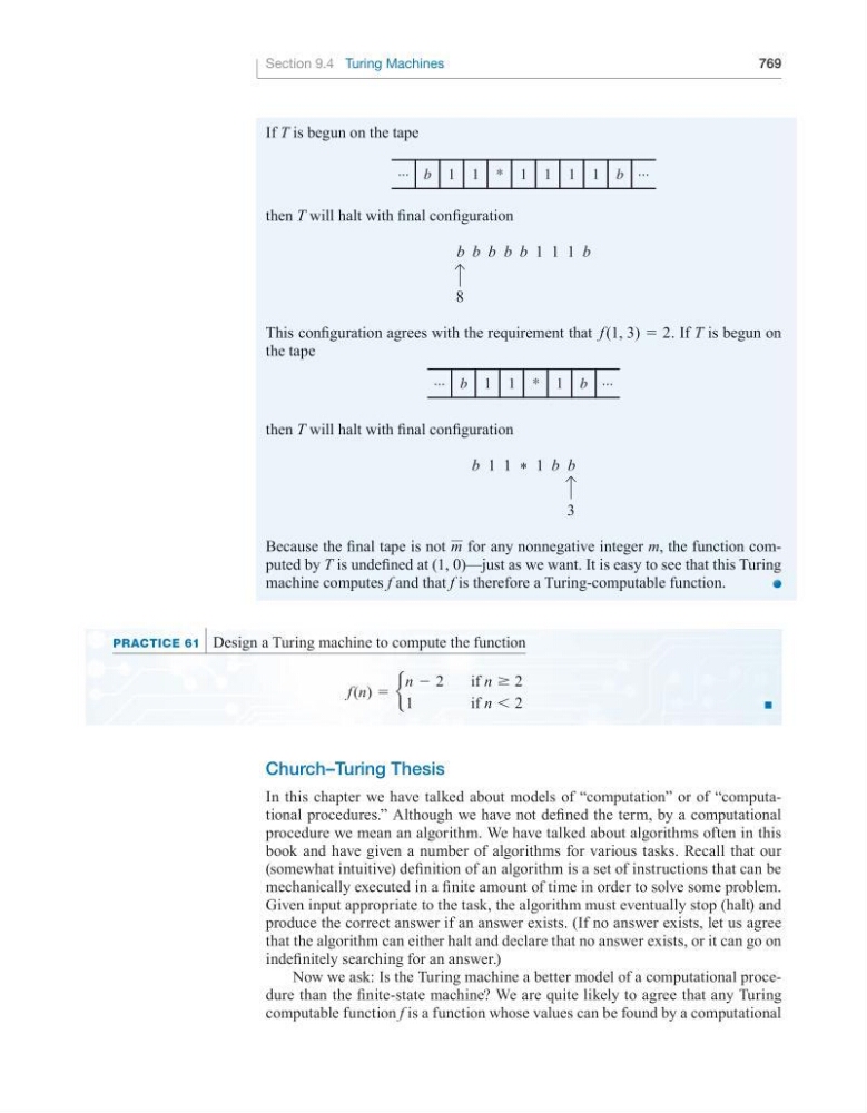
If T is begun on the tape
b
...
1 *
1
1
1 1 1
b ...
then T will halt with final configuration
b b b b b 1 1 1 b
8
This configuration agrees with the requirement that f (1, 3) = 2. If T is begun on
the tape
b
...
*
1 1
1 b ...
then T will halt with final configuration
b 1 1 * 1 b b
3
Because the final tape is not m for any nonnegative integer m, the function computed by T is undefined at (1, 0)—just as we want. It is easy to see that this Turing
machine computes f and that f is therefore a Turing-computable function.
Practice 61 Design a Turing machine to compute the function
f (n) = b
n − 2  if n ≥ 2
1
 if n < 2
■
Church–Turing Thesis
In this chapter we have talked about models of “computation” or of “computational procedures.” Although we have not defined the term, by a computational
procedure we mean an algorithm. We have talked about algorithms often in this
book and have given a number of algorithms for various tasks. Recall that our
(somewhat intuitive) definition of an algorithm is a set of instructions that can be
mechanically executed in a finite amount of time in order to solve some problem.
Given input appropriate to the task, the algorithm must eventually stop (halt) and
produce the correct answer if an answer exists. (If no answer exists, let us agree
that the algorithm can either halt and declare that no answer exists, or it can go on
indefinitely searching for an answer.)
Now we ask: Is the Turing machine a better model of a computational procedure than the finite-state machine? We are quite likely to agree that any Turing
computable function f is a function whose values can be found by a computational