

Section 6.4 Huffman Codes
545
x
y
p
q
(a)
p
y
x
q
(b)
p
q
x
y
p
q
x
(c)
y
(d)
Figure 6.58
(a)
y
T
T '
B '
B
x
(b)
y
x
(c)
frequency f(x) + f(y)
frequency f(x) + f(y)
(d)
Figure 6.59
Now again let f (x) and f ( y) be the minimum frequencies, and suppose we
have a tree T that is optimal for the other frequencies together with the sum
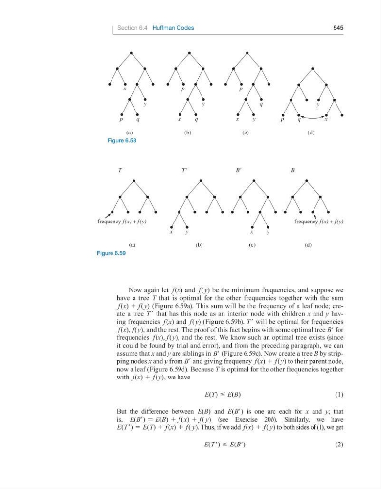
f (x) + f ( y) (Figure 6.59a). This sum will be the frequency of a leaf node; create a tree T ′ that has this node as an interior node with children x and y having frequencies f (x) and f ( y) (Figure 6.59b). T ′ will be optimal for frequencies
f (x), f ( y), and the rest. The proof of this fact begins with some optimal tree B′ for
frequencies f (x), f ( y), and the rest. We know such an optimal tree exists (since
it could be found by trial and error), and from the preceding paragraph, we can
assume that x and y are siblings in B′ (Figure 6.59c). Now create a tree B by stripping nodes x and y from B′ and giving frequency f (x) + f ( y) to their parent node,
now a leaf (Figure 6.59d). Because T is optimal for the other frequencies together
with f (x) + f ( y), we have
E(T) ≤ E(B)
(1)
But the difference between E(B) and E(B′) is one arc each for x and y; that
is, E(B′) = E(B) + f ( x) + f ( y) (see Exercise 20b). Similarly, we have
E(T ′) = E(T) + f (x) + f ( y). Thus, if we add f (x) + f ( y) to both sides of (1), we get
E(T ′) ≤ E(B′)
(2)
545
x
y
p
q
(a)
p
y
x
q
(b)
p
q
x
y
p
q
x
(c)
y
(d)
Figure 6.58
(a)
y
T
T '
B '
B
x
(b)
y
x
(c)
frequency f(x) + f(y)
frequency f(x) + f(y)
(d)
Figure 6.59
Now again let f (x) and f ( y) be the minimum frequencies, and suppose we
have a tree T that is optimal for the other frequencies together with the sum
f (x) + f ( y) (Figure 6.59a). This sum will be the frequency of a leaf node; create a tree T ′ that has this node as an interior node with children x and y having frequencies f (x) and f ( y) (Figure 6.59b). T ′ will be optimal for frequencies
f (x), f ( y), and the rest. The proof of this fact begins with some optimal tree B′ for
frequencies f (x), f ( y), and the rest. We know such an optimal tree exists (since
it could be found by trial and error), and from the preceding paragraph, we can
assume that x and y are siblings in B′ (Figure 6.59c). Now create a tree B by stripping nodes x and y from B′ and giving frequency f (x) + f ( y) to their parent node,
now a leaf (Figure 6.59d). Because T is optimal for the other frequencies together
with f (x) + f ( y), we have
E(T) ≤ E(B)
(1)
But the difference between E(B) and E(B′) is one arc each for x and y; that
is, E(B′) = E(B) + f ( x) + f ( y) (see Exercise 20b). Similarly, we have
E(T ′) = E(T) + f (x) + f ( y). Thus, if we add f (x) + f ( y) to both sides of (1), we get
E(T ′) ≤ E(B′)
(2)