

530
Graphs and Trees
successive comparisons of x to the list items. We have already seen two such algorithms, sequential search and binary search. We can model the activities of these
algorithms by using decision trees. The nodes represent the actions of comparing x
to the list items, where the comparison of x to the ith element in the list is denoted
by x:L3i 4.
Sequential search only distinguishes between two possible outcomes of a comparison of x to L3i 4. If x = L3i 4, the algorithm terminates because x has been found
in the list. If x ∙ L3i 4, the next comparison performed is x:L3i + 1 4, regardless of
whether x was less than or greater than L3i 4. The leaves of this decision tree correspond to the final outcomes, where either x is one of the list items or x is not in the list.
example 32
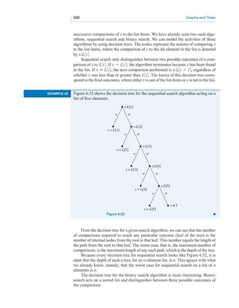
Figure 6.52 shows the decision tree for the sequential search algorithm acting on a
list of five elements.
x:L[1]
x = L[1]
=
≠
x:L[2]
x = L[2]
=
≠
x:L[3]
x = L[3]
=
≠
x:L[4]
x = L[4]
=
≠
x:L[5]
x = L[5]
x ∉L
=
≠
Figure 6.52
From the decision tree for a given search algorithm, we can see that the number
of comparisons required to reach any particular outcome (leaf of the tree) is the
number of internal nodes from the root to that leaf. This number equals the length of
the path from the root to that leaf. The worst case, that is, the maximum number of
comparisons, is the maximum length of any such path, which is the depth of the tree.
Because every decision tree for sequential search looks like Figure 6.52, it is
clear that the depth of such a tree, for an n-element list, is n. This agrees with what
we already know, namely, that the worst case for sequential search on a list of n
elements is n.
The decision tree for the binary search algorithm is more interesting. Binary
search acts on a sorted list and distinguishes between three possible outcomes of
the comparison:
Graphs and Trees
successive comparisons of x to the list items. We have already seen two such algorithms, sequential search and binary search. We can model the activities of these
algorithms by using decision trees. The nodes represent the actions of comparing x
to the list items, where the comparison of x to the ith element in the list is denoted
by x:L3i 4.
Sequential search only distinguishes between two possible outcomes of a comparison of x to L3i 4. If x = L3i 4, the algorithm terminates because x has been found
in the list. If x ∙ L3i 4, the next comparison performed is x:L3i + 1 4, regardless of
whether x was less than or greater than L3i 4. The leaves of this decision tree correspond to the final outcomes, where either x is one of the list items or x is not in the list.
example 32
Figure 6.52 shows the decision tree for the sequential search algorithm acting on a
list of five elements.
x:L[1]
x = L[1]
=
≠
x:L[2]
x = L[2]
=
≠
x:L[3]
x = L[3]
=
≠
x:L[4]
x = L[4]
=
≠
x:L[5]
x = L[5]
x ∉L
=
≠
Figure 6.52
From the decision tree for a given search algorithm, we can see that the number
of comparisons required to reach any particular outcome (leaf of the tree) is the
number of internal nodes from the root to that leaf. This number equals the length of
the path from the root to that leaf. The worst case, that is, the maximum number of
comparisons, is the maximum length of any such path, which is the depth of the tree.
Because every decision tree for sequential search looks like Figure 6.52, it is
clear that the depth of such a tree, for an n-element list, is n. This agrees with what
we already know, namely, that the worst case for sequential search on a list of n
elements is n.
The decision tree for the binary search algorithm is more interesting. Binary
search acts on a sorted list and distinguishes between three possible outcomes of
the comparison: