

492
Graphs and Trees
example 16
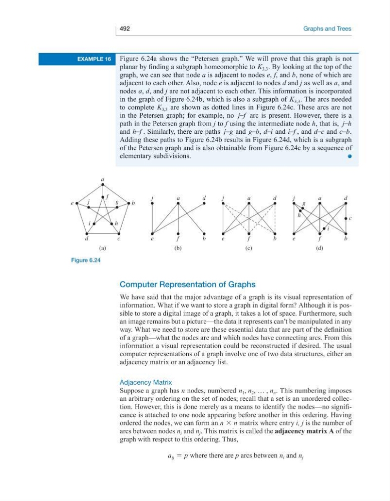
Figure 6.24a shows the “Petersen graph.” We will prove that this graph is not
planar by finding a subgraph homeomorphic to K 3,3 . By looking at the top of the
graph, we can see that node a is adjacent to nodes e, f, and b, none of which are
adjacent to each other. Also, node e is adjacent to nodes d and j as well as a, and
nodes a, d, and j are not adjacent to each other. This information is incorporated
in the graph of Figure 6.24b, which is also a subgraph of K 3,3 . The arcs needed
to complete K 3,3 are shown as dotted lines in Figure 6.24c. These arcs are not
in the Petersen graph; for example, no j–f arc is present. However, there is a
path in the Petersen graph from j to f using the intermediate node h, that is, j–h
and h–f . Similarly, there are paths j–g and g–b, d–i and i–f , and d–c and c–b.
Adding these paths to Figure 6.24b results in Figure 6.24d, which is a subgraph
of the Petersen graph and is also obtainable from Figure 6.24c by a sequence of
elementary subdivisions.
computer representation of Graphs
We have said that the major advantage of a graph is its visual representation of
information. What if we want to store a graph in digital form? Although it is possible to store a digital image of a graph, it takes a lot of space. Furthermore, such
an image remains but a picture—the data it represents can’t be manipulated in any
way. What we need to store are these essential data that are part of the definition
of a graph—what the nodes are and which nodes have connecting arcs. From this
information a visual representation could be reconstructed if desired. The usual
computer representations of a graph involve one of two data structures, either an
adjacency matrix or an adjacency list.
Adjacency Matrix
Suppose a graph has n nodes, numbered n 1 , n 2 , … , n n . This numbering imposes
an arbitrary ordering on the set of nodes; recall that a set is an unordered collection. However, this is done merely as a means to identify the nodes—no significance is attached to one node appearing before another in this ordering. Having
ordered the nodes, we can form an n × n matrix where entry i, j is the number of
arcs between nodes n i and n j . This matrix is called the adjacency matrix a of the
graph with respect to this ordering. Thus,
a ij = p where there are p arcs between n i and n j
a
b
f
e
j
g
d
c
h
i
(a)
j
a
d
e
f
b
(b)
j
a
d
e
f
b
(c)
j g
h
c
a
d
e
f
b
i
(d)
Figure 6.24
Graphs and Trees
example 16
Figure 6.24a shows the “Petersen graph.” We will prove that this graph is not
planar by finding a subgraph homeomorphic to K 3,3 . By looking at the top of the
graph, we can see that node a is adjacent to nodes e, f, and b, none of which are
adjacent to each other. Also, node e is adjacent to nodes d and j as well as a, and
nodes a, d, and j are not adjacent to each other. This information is incorporated
in the graph of Figure 6.24b, which is also a subgraph of K 3,3 . The arcs needed
to complete K 3,3 are shown as dotted lines in Figure 6.24c. These arcs are not
in the Petersen graph; for example, no j–f arc is present. However, there is a
path in the Petersen graph from j to f using the intermediate node h, that is, j–h
and h–f . Similarly, there are paths j–g and g–b, d–i and i–f , and d–c and c–b.
Adding these paths to Figure 6.24b results in Figure 6.24d, which is a subgraph
of the Petersen graph and is also obtainable from Figure 6.24c by a sequence of
elementary subdivisions.
computer representation of Graphs
We have said that the major advantage of a graph is its visual representation of
information. What if we want to store a graph in digital form? Although it is possible to store a digital image of a graph, it takes a lot of space. Furthermore, such
an image remains but a picture—the data it represents can’t be manipulated in any
way. What we need to store are these essential data that are part of the definition
of a graph—what the nodes are and which nodes have connecting arcs. From this
information a visual representation could be reconstructed if desired. The usual
computer representations of a graph involve one of two data structures, either an
adjacency matrix or an adjacency list.
Adjacency Matrix
Suppose a graph has n nodes, numbered n 1 , n 2 , … , n n . This numbering imposes
an arbitrary ordering on the set of nodes; recall that a set is an unordered collection. However, this is done merely as a means to identify the nodes—no significance is attached to one node appearing before another in this ordering. Having
ordered the nodes, we can form an n × n matrix where entry i, j is the number of
arcs between nodes n i and n j . This matrix is called the adjacency matrix a of the
graph with respect to this ordering. Thus,
a ij = p where there are p arcs between n i and n j
a
b
f
e
j
g
d
c
h
i
(a)
j
a
d
e
f
b
(b)
j
a
d
e
f
b
(c)
j g
h
c
a
d
e
f
b
i
(d)
Figure 6.24