

448
Relations, Functions, and Matrices
A more general way to represent arrangements of data is the array. Arrays are
n-dimensional arrangements of data, where n can be any positive integer. If n = 1,
then the data are arranged in a single line, which is therefore a list or finite sequence of data items. This one-dimensional version of an array is called a vector.
If n = 2, the array is a matrix. If n = 3, we can picture layers of two-dimensional
matrices. For n > 3, we can formally deal with the array elements, but we can’t
really visualize the arrangement. The array data structure is available in many
high-level programming languages because it is such a useful way to represent
data in list form or tabular form. Generally, the number of elements expected in
each dimension of the array must be declared in the program. The array X of Example 64, for instance, would be declared as a 3 × 2 array—a two-dimensional
array (matrix) with three elements in one dimension and two in the other (that is,
three rows and two columns).
Matrix operations
Although matrices are particular arrangements of individual elements, we can
treat the matrices themselves as objects, just as we can treat sets of elements as
objects. In each case we are abstracting up one level and looking at the collection
as an entity, rather than looking at the individual elements that make up the collection. We defined operations on sets (union, intersection, and so forth) that made
sets useful for solving counting problems. We can define arithmetic operations on
matrices whose entries are numerical. These operations make matrices interesting
objects to study in their own right, but they also make matrices more useful for
certain tasks such as solving systems of equations.
The first operation, called scalar multiplication, calls for multiplying each
entry of a matrix by a fixed single number called a scalar. The result is a matrix
with the same dimensions as the original matrix.
example 65
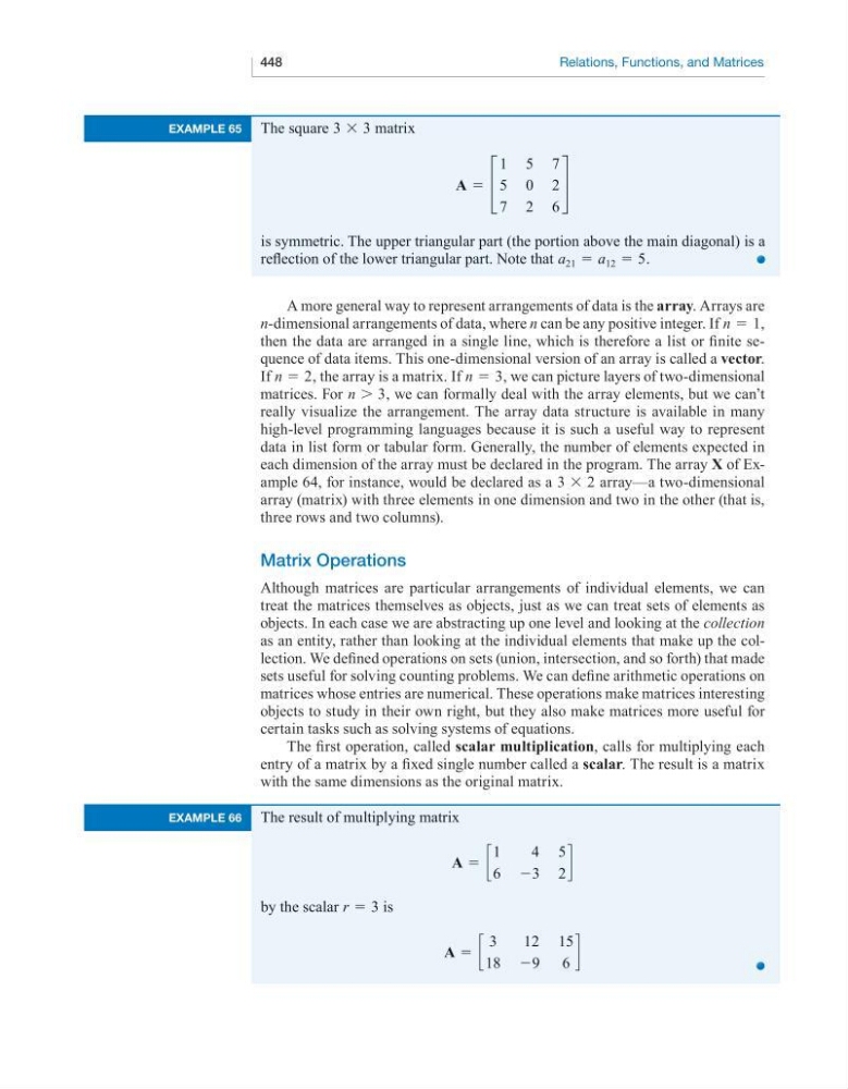
The square 3 × 3 matrix
a = £
1 5 7
5 0 2
7 2 6
§
is symmetric. The upper triangular part (the portion above the main diagonal) is a
reflection of the lower triangular part. Note that a 21 = a 12 = 5.
example 66
The result of multiplying matrix
a = c
1 4 5
6 −3 2
d
by the scalar r = 3 is
a = c
3
12 15
18 −9 6
d
Relations, Functions, and Matrices
A more general way to represent arrangements of data is the array. Arrays are
n-dimensional arrangements of data, where n can be any positive integer. If n = 1,
then the data are arranged in a single line, which is therefore a list or finite sequence of data items. This one-dimensional version of an array is called a vector.
If n = 2, the array is a matrix. If n = 3, we can picture layers of two-dimensional
matrices. For n > 3, we can formally deal with the array elements, but we can’t
really visualize the arrangement. The array data structure is available in many
high-level programming languages because it is such a useful way to represent
data in list form or tabular form. Generally, the number of elements expected in
each dimension of the array must be declared in the program. The array X of Example 64, for instance, would be declared as a 3 × 2 array—a two-dimensional
array (matrix) with three elements in one dimension and two in the other (that is,
three rows and two columns).
Matrix operations
Although matrices are particular arrangements of individual elements, we can
treat the matrices themselves as objects, just as we can treat sets of elements as
objects. In each case we are abstracting up one level and looking at the collection
as an entity, rather than looking at the individual elements that make up the collection. We defined operations on sets (union, intersection, and so forth) that made
sets useful for solving counting problems. We can define arithmetic operations on
matrices whose entries are numerical. These operations make matrices interesting
objects to study in their own right, but they also make matrices more useful for
certain tasks such as solving systems of equations.
The first operation, called scalar multiplication, calls for multiplying each
entry of a matrix by a fixed single number called a scalar. The result is a matrix
with the same dimensions as the original matrix.
example 65
The square 3 × 3 matrix
a = £
1 5 7
5 0 2
7 2 6
§
is symmetric. The upper triangular part (the portion above the main diagonal) is a
reflection of the lower triangular part. Note that a 21 = a 12 = 5.
example 66
The result of multiplying matrix
a = c
1 4 5
6 −3 2
d
by the scalar r = 3 is
a = c
3
12 15
18 −9 6
d