

426
Relations, Functions, and Matrices
example 50
Using the hash function of Example 49, the elements 7, 23, 59, 158 and 48 are
loaded in order into the hash table. The size of the hash table is the same as the
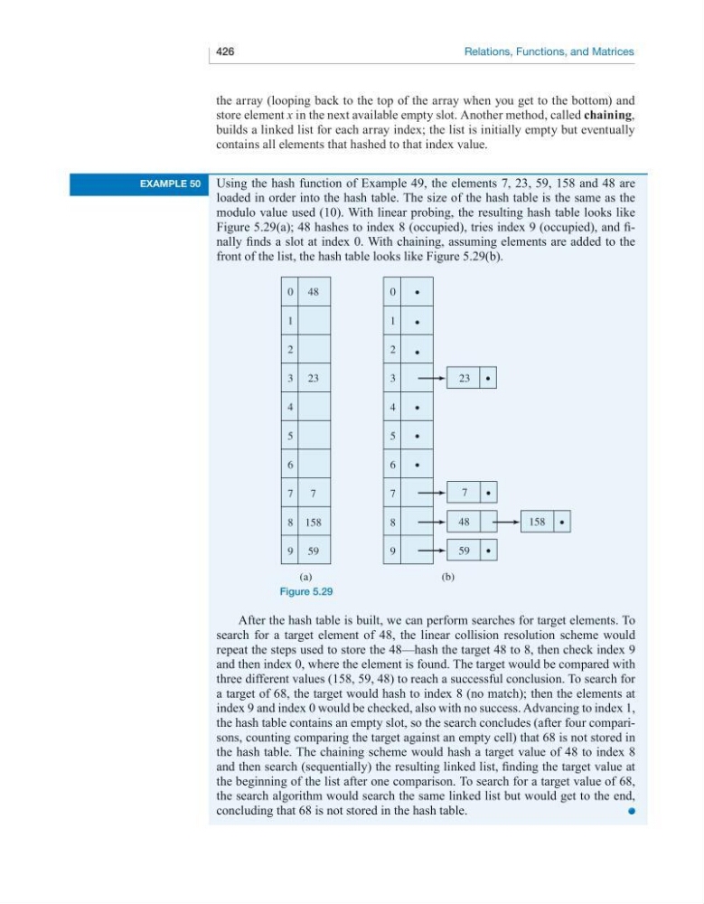
modulo value used (10). With linear probing, the resulting hash table looks like
Figure 5.29(a); 48 hashes to index 8 (occupied), tries index 9 (occupied), and finally finds a slot at index 0. With chaining, assuming elements are added to the
front of the list, the hash table looks like Figure 5.29(b).
0
1
2
3
4
5
6
7
8
9
48
23
7
158
59
(a)
(b)
59
48
158
7
23
0
1
2
3
4
5
6
7
8
9
Figure 5.29
After the hash table is built, we can perform searches for target elements. To
search for a target element of 48, the linear collision resolution scheme would
repeat the steps used to store the 48—hash the target 48 to 8, then check index 9
and then index 0, where the element is found. The target would be compared with
three different values (158, 59, 48) to reach a successful conclusion. To search for
a target of 68, the target would hash to index 8 (no match); then the elements at
index 9 and index 0 would be checked, also with no success. Advancing to index 1,
the hash table contains an empty slot, so the search concludes (after four comparisons, counting comparing the target against an empty cell) that 68 is not stored in
the hash table. The chaining scheme would hash a target value of 48 to index 8
and then search (sequentially) the resulting linked list, finding the target value at
the beginning of the list after one comparison. To search for a target value of 68,
the search algorithm would search the same linked list but would get to the end,
concluding that 68 is not stored in the hash table.
the array (looping back to the top of the array when you get to the bottom) and
store element x in the next available empty slot. Another method, called chaining,
builds a linked list for each array index; the list is initially empty but eventually
contains all elements that hashed to that index value.
Relations, Functions, and Matrices
example 50
Using the hash function of Example 49, the elements 7, 23, 59, 158 and 48 are
loaded in order into the hash table. The size of the hash table is the same as the
modulo value used (10). With linear probing, the resulting hash table looks like
Figure 5.29(a); 48 hashes to index 8 (occupied), tries index 9 (occupied), and finally finds a slot at index 0. With chaining, assuming elements are added to the
front of the list, the hash table looks like Figure 5.29(b).
0
1
2
3
4
5
6
7
8
9
48
23
7
158
59
(a)
(b)
59
48
158
7
23
0
1
2
3
4
5
6
7
8
9
Figure 5.29
After the hash table is built, we can perform searches for target elements. To
search for a target element of 48, the linear collision resolution scheme would
repeat the steps used to store the 48—hash the target 48 to 8, then check index 9
and then index 0, where the element is found. The target would be compared with
three different values (158, 59, 48) to reach a successful conclusion. To search for
a target of 68, the target would hash to index 8 (no match); then the elements at
index 9 and index 0 would be checked, also with no success. Advancing to index 1,
the hash table contains an empty slot, so the search concludes (after four comparisons, counting comparing the target against an empty cell) that 68 is not stored in
the hash table. The chaining scheme would hash a target value of 48 to index 8
and then search (sequentially) the resulting linked list, finding the target value at
the beginning of the list after one comparison. To search for a target value of 68,
the search algorithm would search the same linked list but would get to the end,
concluding that 68 is not stored in the hash table.
the array (looping back to the top of the array when you get to the bottom) and
store element x in the next available empty slot. Another method, called chaining,
builds a linked list for each array index; the list is initially empty but eventually
contains all elements that hashed to that index value.