

382
Relations, Functions, and Matrices
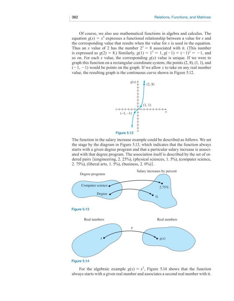
Of course, we also use mathematical functions in algebra and calculus. The
equation g(x) = x
3
expresses a functional relationship between a value for x and
the corresponding value that results when the value for x is used in the equation.
Thus an x value of 2 has the number 2
3
= 8 associated with it. (This number
is expressed as g(2) = 8.) Similarly, g(1) = 1
3
= 1, g(−1) = (−1)
3
= −1, and
so on. For each x value, the corresponding g(x) value is unique. If we were to
graph this function on a rectangular coordinate system, the points (2, 8), (1, 1), and
(−1, −1) would be points on the graph. If we allow x to take on any real number
value, the resulting graph is the continuous curve shown in Figure 5.12.
(–1, –1)
(1, 1)
(2, 8)
g(x)
x
The function in the salary increase example could be described as follows. We set
the stage by the diagram in Figure 5.13, which indicates that the function always
starts with a given degree program and that a particular salary increase is associated with that degree program. The association itself is described by the set of ordered pairs 5(engineering, 2. 25%), (physical sciences, 1. 5%), (computer science,
2. 75%), (liberal arts, 1. 5%), (business, 2. 0%)6.
Computer science
Degree
%
2.75%
Real numbers
Real numbers
g(x)
g
x
For the algebraic example g(x) = x
3
, Figure 5.14 shows that the function
always starts with a given real number and associates a second real number with it.
Figure 5.12
Figure 5.13
Figure 5.14
Degree programs
Salary increases by percent
Relations, Functions, and Matrices
Of course, we also use mathematical functions in algebra and calculus. The
equation g(x) = x
3
expresses a functional relationship between a value for x and
the corresponding value that results when the value for x is used in the equation.
Thus an x value of 2 has the number 2
3
= 8 associated with it. (This number
is expressed as g(2) = 8.) Similarly, g(1) = 1
3
= 1, g(−1) = (−1)
3
= −1, and
so on. For each x value, the corresponding g(x) value is unique. If we were to
graph this function on a rectangular coordinate system, the points (2, 8), (1, 1), and
(−1, −1) would be points on the graph. If we allow x to take on any real number
value, the resulting graph is the continuous curve shown in Figure 5.12.
(–1, –1)
(1, 1)
(2, 8)
g(x)
x
The function in the salary increase example could be described as follows. We set
the stage by the diagram in Figure 5.13, which indicates that the function always
starts with a given degree program and that a particular salary increase is associated with that degree program. The association itself is described by the set of ordered pairs 5(engineering, 2. 25%), (physical sciences, 1. 5%), (computer science,
2. 75%), (liberal arts, 1. 5%), (business, 2. 0%)6.
Computer science
Degree
%
2.75%
Real numbers
Real numbers
g(x)
g
x
For the algebraic example g(x) = x
3
, Figure 5.14 shows that the function
always starts with a given real number and associates a second real number with it.
Figure 5.12
Figure 5.13
Figure 5.14
Degree programs
Salary increases by percent