

304
Sets, Combinatorics, and Probability
Using our definition
P(E) =
0 E 0
0 S 0
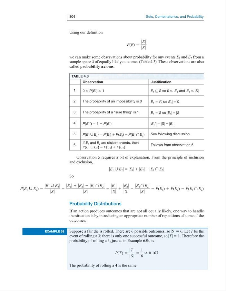
we can make some observations about probability for any events E 1 and E 2 from a
sample space S of equally likely outcomes (Table 4.3). These observations are also
called probability axioms.
Table 4.3
Observation
Justification
1.
0 ≤ P( E 1 ) ≤ 1
E 1 # S so 0 ≤ 0 E 1 0 and 0 E 1 0 ≤ 0 S 0
2.
The probability of an impossibility is 0
E 1 = [ so 0 E 1 0 = 0
3.
The probability of a “sure thing” is 1
E 1 = S so 0 E 1 0 = 0 S 0
4.
P( E 1 ′) = 1 − P( E 1 )
0 E 1 ′0 = 0 S 0 − 0 E 1 0
5.
P( E 1 c E 2 ) = P( E 1 ) + P( E 2 ) − P( E 1 d E 2 )
See following discussion
6.
If E 1 and E 2 are disjoint events, then
P( E 1 c E 2 ) = P( E 1 ) + P( E 2 )
Follows from observation 5
Observation 5 requires a bit of explanation. From the principle of inclusion
and exclusion,
0 E 1 c E 2 0 = 0 E 1 0 + 0 E 2 0 − 0 E 1 d E 2 0
So
P(E 1 c E 2 ) =
0 E 1 c E 2 0
0 S 0
=
0 E 1 0 + 0 E 2 0 − 0 E 1 d E 2 0
0 S 0
=
0 E 1 0
0 S 0
+
0 E 2 0
0 S 0
−
0 E 1 d E 2 0
0 S 0
= P(E 1 ) + P(E 2 ) − P(E 1 d E 2 )
Probability Distributions
If an action produces outcomes that are not all equally likely, one way to handle
the situation is by introducing an appropriate number of repetitions of some of the
outcomes.
example 69
Suppose a fair die is rolled. There are 6 possible outcomes, so 0 S 0 = 6. Let T be the
event of rolling a 3; there is only one successful outcome, so 0 T 0 = 1. Therefore the
probability of rolling a 3, just as in Example 65b, is
P(T ) =
0 T 0
0 S 0
=
1
6
> 0.167
The probability of rolling a 4 is the same.
Sets, Combinatorics, and Probability
Using our definition
P(E) =
0 E 0
0 S 0
we can make some observations about probability for any events E 1 and E 2 from a
sample space S of equally likely outcomes (Table 4.3). These observations are also
called probability axioms.
Table 4.3
Observation
Justification
1.
0 ≤ P( E 1 ) ≤ 1
E 1 # S so 0 ≤ 0 E 1 0 and 0 E 1 0 ≤ 0 S 0
2.
The probability of an impossibility is 0
E 1 = [ so 0 E 1 0 = 0
3.
The probability of a “sure thing” is 1
E 1 = S so 0 E 1 0 = 0 S 0
4.
P( E 1 ′) = 1 − P( E 1 )
0 E 1 ′0 = 0 S 0 − 0 E 1 0
5.
P( E 1 c E 2 ) = P( E 1 ) + P( E 2 ) − P( E 1 d E 2 )
See following discussion
6.
If E 1 and E 2 are disjoint events, then
P( E 1 c E 2 ) = P( E 1 ) + P( E 2 )
Follows from observation 5
Observation 5 requires a bit of explanation. From the principle of inclusion
and exclusion,
0 E 1 c E 2 0 = 0 E 1 0 + 0 E 2 0 − 0 E 1 d E 2 0
So
P(E 1 c E 2 ) =
0 E 1 c E 2 0
0 S 0
=
0 E 1 0 + 0 E 2 0 − 0 E 1 d E 2 0
0 S 0
=
0 E 1 0
0 S 0
+
0 E 2 0
0 S 0
−
0 E 1 d E 2 0
0 S 0
= P(E 1 ) + P(E 2 ) − P(E 1 d E 2 )
Probability Distributions
If an action produces outcomes that are not all equally likely, one way to handle
the situation is by introducing an appropriate number of repetitions of some of the
outcomes.
example 69
Suppose a fair die is rolled. There are 6 possible outcomes, so 0 S 0 = 6. Let T be the
event of rolling a 3; there is only one successful outcome, so 0 T 0 = 1. Therefore the
probability of rolling a 3, just as in Example 65b, is
P(T ) =
0 T 0
0 S 0
=
1
6
> 0.167
The probability of rolling a 4 is the same.