

Section 3.2 Recurrence Relations
193
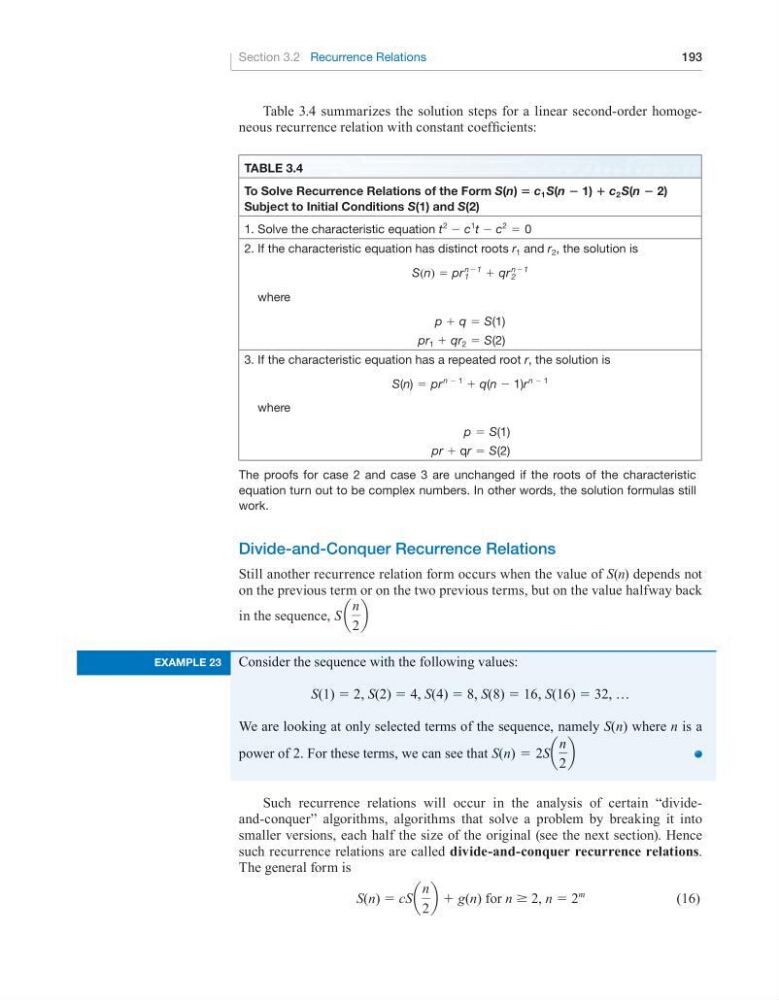
Table 3.4 summarizes the solution steps for a linear second-order homogeneous recurrence relation with constant coefficients:
Divide-and-Conquer Recurrence Relations
Still another recurrence relation form occurs when the value of S(n) depends not
on the previous term or on the two previous terms, but on the value halfway back
in the sequence, S a
n
2
b
table 3.4
to Solve recurrence relations of the Form S(n) ∙ c 1 S(n ∙ 1) ∙ c 2 S(n ∙ 2)
Subject to Initial conditions S(1) and S(2)
1. Solve the characteristic equation t
2
− c
1
t − c
2
= 0
2. If the characteristic equation has distinct roots r 1 and r 2 , the solution is
S(n) = pr
n−1
1
+ qr
n−1
2
where
p + q = S(1)
pr 1 + qr 2 = S(2)
3. If the characteristic equation has a repeated root r, the solution is
S(n) = pr
n − 1
+ q(n − 1)r
n − 1
where
p = S(1)
pr + qr = S(2)
The proofs for case 2 and case 3 are unchanged if the roots of the characteristic
equation turn out to be complex numbers. In other words, the solution formulas still
work.
Such recurrence relations will occur in the analysis of certain “divideand-conquer” algorithms, algorithms that solve a problem by breaking it into
smaller versions, each half the size of the original (see the next section). Hence
such recurrence relations are called divide-and-conquer recurrence relations.
The general form is
S(n) = cS a
n
2
b + g(n) for n ≥ 2, n = 2
m
(16)
example 23
Consider the sequence with the following values:
S(1) = 2, S(2) = 4, S(4) = 8, S(8) = 16, S(16) = 32, …
We are looking at only selected terms of the sequence, namely S(n) where n is a
power of 2. For these terms, we can see that S(n) = 2Sa
n
2
b
193
Table 3.4 summarizes the solution steps for a linear second-order homogeneous recurrence relation with constant coefficients:
Divide-and-Conquer Recurrence Relations
Still another recurrence relation form occurs when the value of S(n) depends not
on the previous term or on the two previous terms, but on the value halfway back
in the sequence, S a
n
2
b
table 3.4
to Solve recurrence relations of the Form S(n) ∙ c 1 S(n ∙ 1) ∙ c 2 S(n ∙ 2)
Subject to Initial conditions S(1) and S(2)
1. Solve the characteristic equation t
2
− c
1
t − c
2
= 0
2. If the characteristic equation has distinct roots r 1 and r 2 , the solution is
S(n) = pr
n−1
1
+ qr
n−1
2
where
p + q = S(1)
pr 1 + qr 2 = S(2)
3. If the characteristic equation has a repeated root r, the solution is
S(n) = pr
n − 1
+ q(n − 1)r
n − 1
where
p = S(1)
pr + qr = S(2)
The proofs for case 2 and case 3 are unchanged if the roots of the characteristic
equation turn out to be complex numbers. In other words, the solution formulas still
work.
Such recurrence relations will occur in the analysis of certain “divideand-conquer” algorithms, algorithms that solve a problem by breaking it into
smaller versions, each half the size of the original (see the next section). Hence
such recurrence relations are called divide-and-conquer recurrence relations.
The general form is
S(n) = cS a
n
2
b + g(n) for n ≥ 2, n = 2
m
(16)
example 23
Consider the sequence with the following values:
S(1) = 2, S(2) = 4, S(4) = 8, S(8) = 16, S(16) = 32, …
We are looking at only selected terms of the sequence, namely S(n) where n is a
power of 2. For these terms, we can see that S(n) = 2Sa
n
2
b