

Time Domain Representation of Continuous and Discrete Signals
63
subplot(2,2,1);
stem (n, real(fn)); hold on; plot(n,yzero);
title (‘real part of [f(n)] vs. n’)
ylabel(‘real part of [f(n)]’);
axis([0 15 -2 3])
subplot(2,2,2);
stem(n, imag(fn));
hold on;plot(n,yzero);
ylabel(‘imaginary part of [f(n)]’)
title(‘imaginary part of [f(n)] vs. n’)
ylabel(‘imaginary part of [f(n)]’);
axis([0 15 -2 2])
subplot(2,2,3);
stem(n, abs(fn));
title(‘magnitude of [f(n)] vs. n’)
xlabel(‘time index n’)
ylabel(‘magnitude of [f(n)]’)
subplot(2,2,4);
stem(n,(180/pi) * angle(fn));
hold on; plot(n,yzero);
title(‘phase of [f(n)] vs n’)
xlabel(‘time index n’)
ylabel(‘degrees’)
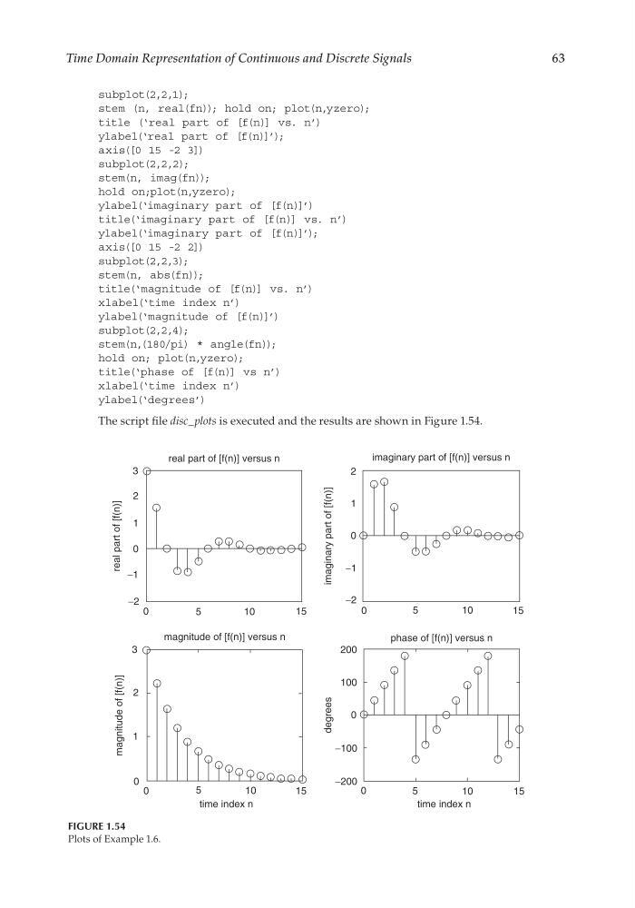
The script fi le disc_plots is executed and the results are shown in Figure 1.54.
real part of [f(n)] versus n
imaginary part of [f(n)] versus n
real part of [f(n)]
imaginary part of [f(n)]
3
2
1
−1
−2
0
5
1 0
15
0
2
0
−1
−2
0
5
1 0
15
1
magnitude of [f(n)] versus n
3
2
1
0
0
5
10
15
magnitude of [f(n)]
time index n
time index n
degrees
200
100
−100
−200
0
0
5
10
15
phase of [f(n)] versus n
FIGURE 1.54
Plots of Example 1.6.
CRC_47760_CH001.indd 63
CRC_47760_CH001.indd 63
7/25/2008 4:16:23 PM
7/25/2008 4:16:23 PM
63
subplot(2,2,1);
stem (n, real(fn)); hold on; plot(n,yzero);
title (‘real part of [f(n)] vs. n’)
ylabel(‘real part of [f(n)]’);
axis([0 15 -2 3])
subplot(2,2,2);
stem(n, imag(fn));
hold on;plot(n,yzero);
ylabel(‘imaginary part of [f(n)]’)
title(‘imaginary part of [f(n)] vs. n’)
ylabel(‘imaginary part of [f(n)]’);
axis([0 15 -2 2])
subplot(2,2,3);
stem(n, abs(fn));
title(‘magnitude of [f(n)] vs. n’)
xlabel(‘time index n’)
ylabel(‘magnitude of [f(n)]’)
subplot(2,2,4);
stem(n,(180/pi) * angle(fn));
hold on; plot(n,yzero);
title(‘phase of [f(n)] vs n’)
xlabel(‘time index n’)
ylabel(‘degrees’)
The script fi le disc_plots is executed and the results are shown in Figure 1.54.
real part of [f(n)] versus n
imaginary part of [f(n)] versus n
real part of [f(n)]
imaginary part of [f(n)]
3
2
1
−1
−2
0
5
1 0
15
0
2
0
−1
−2
0
5
1 0
15
1
magnitude of [f(n)] versus n
3
2
1
0
0
5
10
15
magnitude of [f(n)]
time index n
time index n
degrees
200
100
−100
−200
0
0
5
10
15
phase of [f(n)] versus n
FIGURE 1.54
Plots of Example 1.6.
CRC_47760_CH001.indd 63
CRC_47760_CH001.indd 63
7/25/2008 4:16:23 PM
7/25/2008 4:16:23 PM