

58
Practical MATLAB
® Applications for Engineers
1.4 Examples
Example 1.1
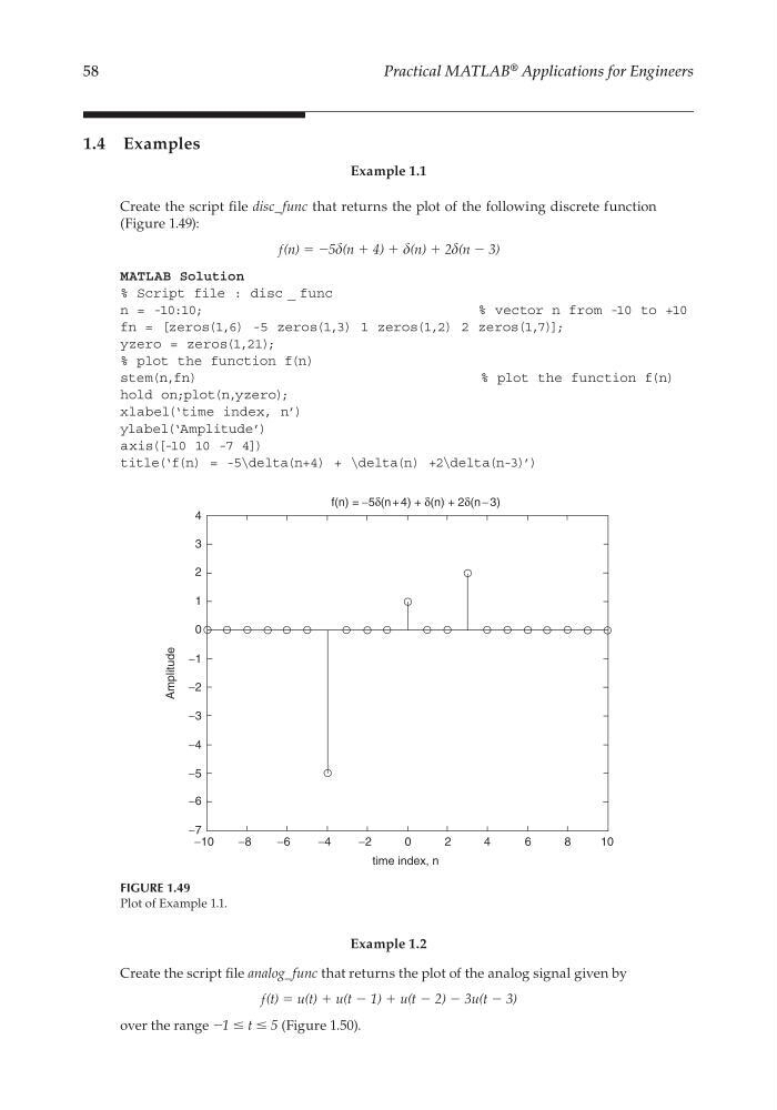
Create the script fi le disc_func that returns the plot of the following discrete function
(Figure 1.49):
ƒ(n) = −5(n + 4) + (n) + 2(n − 3)
MATLAB Solution
% Script file : disc _ func
n = -10:10;
% vector n from -10 to +10
fn = [zeros(1,6) -5 zeros(1,3) 1 zeros(1,2) 2 zeros(1,7)];
yzero = zeros(1,21);
% plot the function f(n)
stem(n,fn)
% plot the function f(n)
hold on;plot(n,yzero);
xlabel(‘time index, n’)
ylabel(‘Amplitude’)
axis([-10 10 -7 4])
title(‘f(n) = -5\delta(n+4) + \delta(n) +2\delta(n-3)’)
Example 1.2
Create the script fi le analog_func that returns the plot of the analog signal given by
ƒ(t) = u(t) + u(t − 1) + u(t − 2) − 3u(t − 3)
over the range −1 ≤ t ≤ 5 (Figure 1.50).
f(n) = −5δ(n + 4) + δ(n) + 2δ(n − 3)
4
3
2
1
−1
−2
−3
−4
−5
−6
−10
−8
−6
−4
−2
0
2
4
6
8
1 0
−7
0
time index, n
Amplitude
FIGURE 1.49
Plot of Example 1.1.
CRC_47760_CH001.indd 58
CRC_47760_CH001.indd 58
7/25/2008 4:16:22 PM
7/25/2008 4:16:22 PM
Practical MATLAB
® Applications for Engineers
1.4 Examples
Example 1.1
Create the script fi le disc_func that returns the plot of the following discrete function
(Figure 1.49):
ƒ(n) = −5(n + 4) + (n) + 2(n − 3)
MATLAB Solution
% Script file : disc _ func
n = -10:10;
% vector n from -10 to +10
fn = [zeros(1,6) -5 zeros(1,3) 1 zeros(1,2) 2 zeros(1,7)];
yzero = zeros(1,21);
% plot the function f(n)
stem(n,fn)
% plot the function f(n)
hold on;plot(n,yzero);
xlabel(‘time index, n’)
ylabel(‘Amplitude’)
axis([-10 10 -7 4])
title(‘f(n) = -5\delta(n+4) + \delta(n) +2\delta(n-3)’)
Example 1.2
Create the script fi le analog_func that returns the plot of the analog signal given by
ƒ(t) = u(t) + u(t − 1) + u(t − 2) − 3u(t − 3)
over the range −1 ≤ t ≤ 5 (Figure 1.50).
f(n) = −5δ(n + 4) + δ(n) + 2δ(n − 3)
4
3
2
1
−1
−2
−3
−4
−5
−6
−10
−8
−6
−4
−2
0
2
4
6
8
1 0
−7
0
time index, n
Amplitude
FIGURE 1.49
Plot of Example 1.1.
CRC_47760_CH001.indd 58
CRC_47760_CH001.indd 58
7/25/2008 4:16:22 PM
7/25/2008 4:16:22 PM