650
Practical MATLAB
® Applications for Engineers
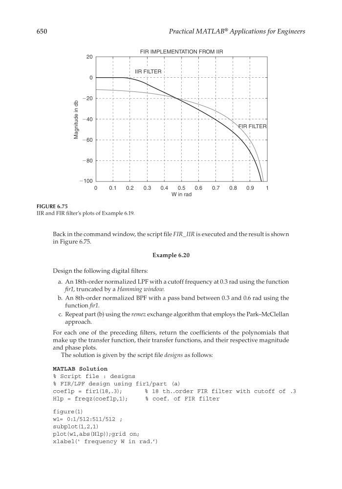
Back in the command window, the script fi le FIR_IIR is executed and the result is shown
in Figure 6.75.
Example 6.20
Design the following digital fi lters:
a. An 18th-order normalized LPF with a cutoff frequency at 0.3 rad using the function
fi r1, truncated by a Hamming window.
b. An 8th-order normalized BPF with a pass band between 0.3 and 0.6 rad using the
function fi r1.
c. Repeat part (b) using the remez exchange algorithm that employs the Park–McClellan
approach.
For each one of the preceding fi lters, return the coeffi cients of the polynomials that
make up the transfer function, their transfer functions, and their respective magnitude
and phase plots.
The solution is given by the script fi le designs as follows:
MATLAB Solution
% Script file : designs
% FIR/LPF design using fir1/part (a)
coeflp = fir1(18,.3);
% 18 th..order FIR filter with cutoff of .3
Hlp = freqz(coeflp,1);
% coef. of FIR filter
figure(1)
w1= 0:1/512:511/512 ;
subplot(1,2,1)
plot(w1,abs(Hlp));grid on;
xlabel(‘ frequency W in rad.’)
FIGURE 6.75
IIR and FIR fi lter’s plots of Example 6.19.
20
FIR IMPLEMENTATION FROM IIR
0
Ϫ20
Ϫ40
Ϫ60
Ϫ80
Ϫ100
0
0.1
0.2
0.3
0.4
0.5
W in rad
0.6
0.7
0.8
0.9
1
Magnitude in db
IIR FILTER
FIR FILTER
CRC_47760_CH006.indd 650
CRC_47760_CH006.indd 650
7/23/2008 2:27:00 PM
7/23/2008 2:27:00 PM