

Time Domain Representation of Continuous and Discrete Signals
55
MATLAB Solution
% Script file: audio
subplot(2,1,1)
fo = 1000;
Fs = 8000;Ts =1/Fs;
t = 0:Ts:1;
y = cos(2*pi*fo.*t)+3*cos(0.5*pi*fo.*t);
% audio sequence
plot(t(1:100),y(1:100));
ylabel(‘Amplitude’);
xlabel(‘time (sec)’);
title(‘cos(2\pi fo t)+3 cos(0.5\pi fo t) vs.t ‘)
subplot(2,1,2)
load mtlb; Fs=1418; T=1/Fs;
x = 1:4001;xx=x.*T;
% speech file
plot(xx,mtlb);
axis([0 4000*T -4 4]);
ylabel(‘Amplitude ‘);
title(‘[Speech file mtlb] vs. t’);
xlabel(‘time (sec)’)
R.1.167 The MATLAB command [y, Fs, nbits] = wavread(‘microsoft_fi le’) returns the vector y
consisting of the audio wave samples from a Microsoft fi le, at a sampling frequency
Fs, using n bits to encode each sample of y, whereas the amplitude of y is scaled
over the range −1 ≤ y ≤ +1. Similarly, the command wavwrite returns a Microsoft
wave fi le.
R.1.168 The MATLAB command image(matrix_A) returns matrix_A as an image, where
each element of the matrix_A is defi ned by a color. The matrix dimensions may
be 2-D (m × n) or 3-D (m × n × r). In its simplest version, the elements of the 2-D
(n × m) matrix are used as indices in the current colormap to defi ne its color.
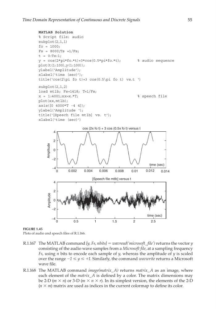
FIGURE 1.45
Plots of audio and speech fi les of R.1.166.
cos (2π fo t) + 3 cos (0.5π fo t) versus t
4
2
0
−2
−4
0
0.002
0.004
0.006
0.008
0.01
0.012
0.014
time (sec)
time (sec)
[Speech file mtlb] versus t
4
2
0
−2
−4
0
0.5
1
1.5
2
2.5
Amplitude
Amplitude
CRC_47760_CH001.indd 55
CRC_47760_CH001.indd 55
7/25/2008 4:16:20 PM
7/25/2008 4:16:20 PM
55
MATLAB Solution
% Script file: audio
subplot(2,1,1)
fo = 1000;
Fs = 8000;Ts =1/Fs;
t = 0:Ts:1;
y = cos(2*pi*fo.*t)+3*cos(0.5*pi*fo.*t);
% audio sequence
plot(t(1:100),y(1:100));
ylabel(‘Amplitude’);
xlabel(‘time (sec)’);
title(‘cos(2\pi fo t)+3 cos(0.5\pi fo t) vs.t ‘)
subplot(2,1,2)
load mtlb; Fs=1418; T=1/Fs;
x = 1:4001;xx=x.*T;
% speech file
plot(xx,mtlb);
axis([0 4000*T -4 4]);
ylabel(‘Amplitude ‘);
title(‘[Speech file mtlb] vs. t’);
xlabel(‘time (sec)’)
R.1.167 The MATLAB command [y, Fs, nbits] = wavread(‘microsoft_fi le’) returns the vector y
consisting of the audio wave samples from a Microsoft fi le, at a sampling frequency
Fs, using n bits to encode each sample of y, whereas the amplitude of y is scaled
over the range −1 ≤ y ≤ +1. Similarly, the command wavwrite returns a Microsoft
wave fi le.
R.1.168 The MATLAB command image(matrix_A) returns matrix_A as an image, where
each element of the matrix_A is defi ned by a color. The matrix dimensions may
be 2-D (m × n) or 3-D (m × n × r). In its simplest version, the elements of the 2-D
(n × m) matrix are used as indices in the current colormap to defi ne its color.
FIGURE 1.45
Plots of audio and speech fi les of R.1.166.
cos (2π fo t) + 3 cos (0.5π fo t) versus t
4
2
0
−2
−4
0
0.002
0.004
0.006
0.008
0.01
0.012
0.014
time (sec)
time (sec)
[Speech file mtlb] versus t
4
2
0
−2
−4
0
0.5
1
1.5
2
2.5
Amplitude
Amplitude
CRC_47760_CH001.indd 55
CRC_47760_CH001.indd 55
7/25/2008 4:16:20 PM
7/25/2008 4:16:20 PM