646
Practical MATLAB
® Applications for Engineers
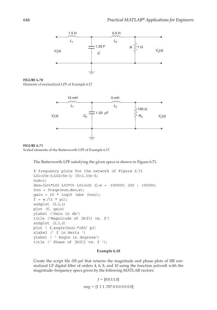
The Butterworth LPF satisfying the given specs is shown in Figure 6.71.
% frequency plots for the network of Figure 6.71
L01=15e-3;L02=5e-3; C0=1.33e-6;
num=1;
den=[L01*L02 L01*C0 L01+L02 1];w = -155000: 250 : 155000;
hnn = freqs(num,den,w);
gain = 20 * log10 (abs (hnn));
f = w./(2 * pi);
subplot (2,1,1)
plot (f, gain)
ylabel (‘Gain in db’)
title (‘Magnitude of [H(f)] vs. f’)
subplot (2,1,2)
plot ( f,angle(hnn).*180/ pi)
xlabel (‘ f in Hertz ’)
ylabel ( ‘ Angle in degrees’)
title (‘ Phase of [H(f)] vs. f ’);
Example 6.18
Create the script fi le IIR-yul that returns the magnitude and phase plots of IIR normalized LP digital fi lter of orders 4, 6, 8, and 10 using the function yulewalk with the
magnitude–frequency specs given by the following MATLAB vectors:
f = [0:0.1:1.0]
mag = [1 1 1 .707 0 0 0 0 0 0 0]
FIGURE 6.70
Elements of normalized LPF of Example 6.17.
1.5 H
1.33 F
0.5 H
1 Ω
V o (s)
V i (s)
L 1
C
L 2
R
FIGURE 6.71
Scaled elements of the Butterworth LPF of Example 6.17.
15 mH
1.33 µF
5 mH
100 Ω
V i (s)
V o (s)
L 1
C 0
L 2
R 0
CRC_47760_CH006.indd 646
CRC_47760_CH006.indd 646
7/23/2008 2:26:59 PM
7/23/2008 2:26:59 PM