Analog and Digital Filters
643
Example 6.17
Create the script fi le butt_implem that returns a third-order analog Butterworth LPF, at
the component level, with w c = 10
4 rad/s and a load impedance of 100 Ω.
a. Start the design with a third-order normalized prototype LPF and obtain the corresponding magnitude and phase plots.
b. Obtain the corresponding transfer function coeffi cients and the system poles (check
for stability).
c. Obtain the normalized fi lter’s transfer function.
d. Use frequency and magnitude scaling to obtain the desired fi lter transfer function.
ANALYTICAL Solution
The structure chosen for the desired LP normalized, third-order fi lter prototype (see
R.6.49) is the π section shown in Figure 6.68.
The transfer function is indicated as follows:
H s
L L C s
L C s
L
L s
N ( )
(
)
(
)
(
)
ϭ
ϩ
ϩ
ϩ
ϩ
1
1
1 2
3
1
2
1
2
(6.3)
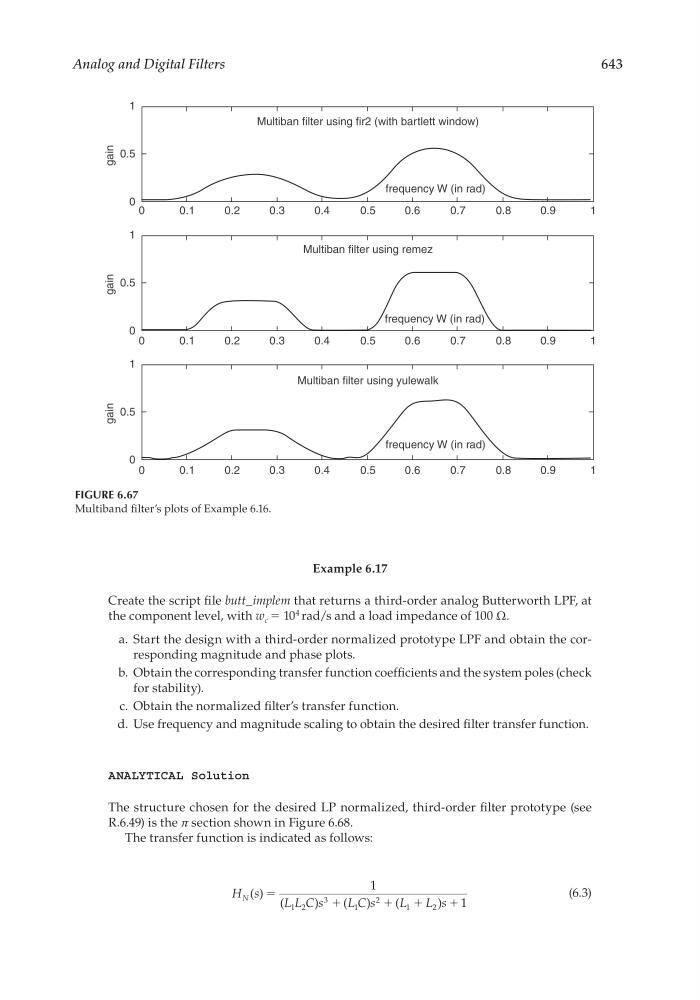
FIGURE 6.67
Multiband fi lter’s plots of Example 6.16.
1
0.5
0
0
0.1
gain
0.2
0.3
0.4
0.5
Multiban filter using fir2 (with bartlett window)
Multiban filter using remez
Multiban filter using yulewalk
frequency W (in rad)
frequency W (in rad)
frequency W (in rad)
0.6
0.7
0.8
1
0.9
1
0.5
0
0
0.1
gain
0.2
0.3
0.4
0.5
0.6
0.7
0.8
1
0.9
1
0.5
0
0
0.1
gain
0.2
0.3
0.4
0.5
0.6
0.7
0.8
1
0.9
CRC_47760_CH006.indd 643
CRC_47760_CH006.indd 643
7/23/2008 2:26:57 PM
7/23/2008 2:26:57 PM