620
Practical MATLAB
® Applications for Engineers
Example 6.5
Let H s
V s
V s
a s
a s
o
i
( )
( )
( )
ϭ
ϭ
ϩ
ϩ
2
2
1
1
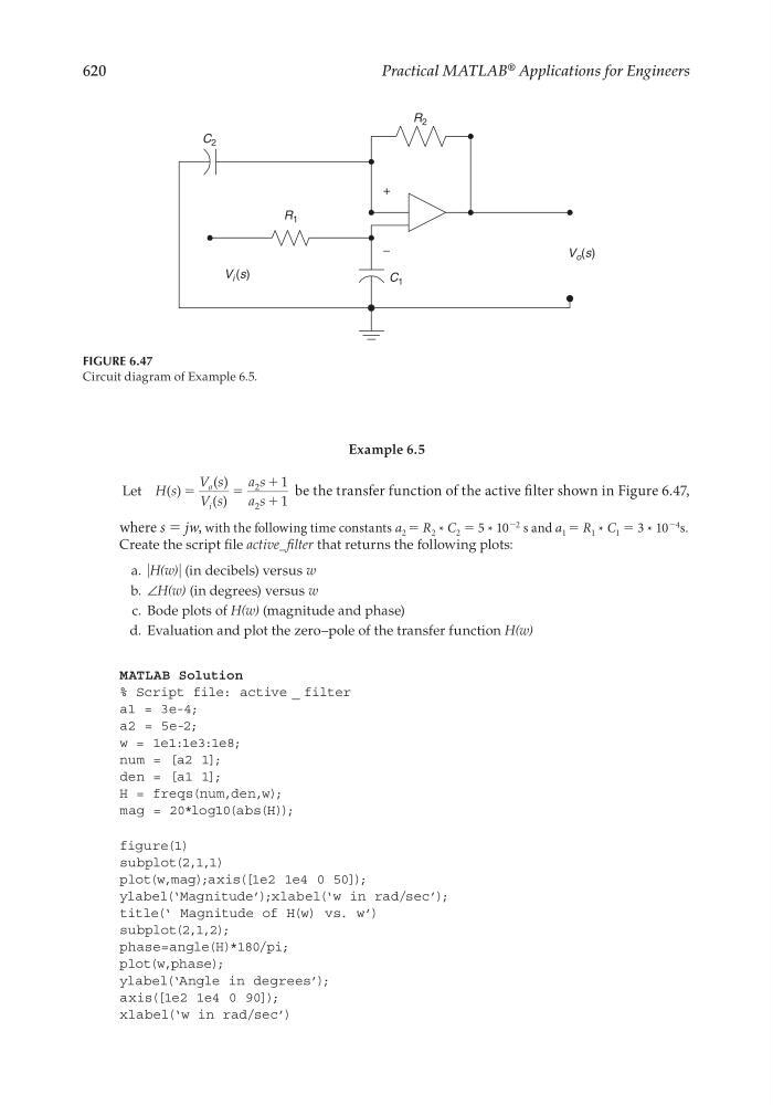
be the transfer function of the active fi lter shown in Figure 6.47,
where s = jw, with the following time constants a 2 = R 2 * C 2 = 5 * 10
−2 s and a 1 = R 1 * C 1 = 3 * 10
−4 s.
Create the script fi le active_fi lter that returns the following plots:
a. ͉H(w)͉ (in decibels) versus w
b. ∠H(w) (in degrees) versus w
c. Bode plots of H(w) (magnitude and phase)
d. Evaluation and plot the zero–pole of the transfer function H(w)
MATLAB Solution
% Script file: active _ filter
a1 = 3e-4;
a2 = 5e-2;
w = 1e1:1e3:1e8;
num = [a2 1];
den = [a1 1];
H = freqs(num,den,w);
mag = 20*log10(abs(H));
figure(1)
subplot(2,1,1)
plot(w,mag);axis([1e2 1e4 0 50]);
ylabel(‘Magnitude’);xlabel(‘w in rad/sec’);
title(‘ Magnitude of H(w) vs. w’)
subplot(2,1,2);
phase=angle(H)*180/pi;
plot(w,phase);
ylabel(‘Angle in degrees’);
axis([1e2 1e4 0 90]);
xlabel(‘w in rad/sec’)
FIGURE 6.47
Circuit diagram of Example 6.5.
C 2
C 1
V i (s)
V o (s)
R 1
R 2
+
−
CRC_47760_CH006.indd 620
CRC_47760_CH006.indd 620
7/23/2008 2:26:49 PM
7/23/2008 2:26:49 PM