552
Practical MATLAB
® Applications for Engineers
0
2.3000
-6.3250
54.6006
-192.4085
38.0520
****************************
Coefficients of the denominator polynomial of H(z)
1.0000
-2.1700
1.8366
-0.1757
-0.4300
0.1169
***************************
The first 11 coefficients of the impulse response h(n) are:
***************************
coef. num.
h(n)
***************************
ans =
0
0
1.0000
2.3000
2.0000
-1.3340
3.0000
47.4817
4.0000
-86.5192
5.0000
-236.1448
6.0000
-346.0348
7.0000
-311.8158
8.0000
-125.3485
9.0000
148.4517
10.0000
376.3726
***************************
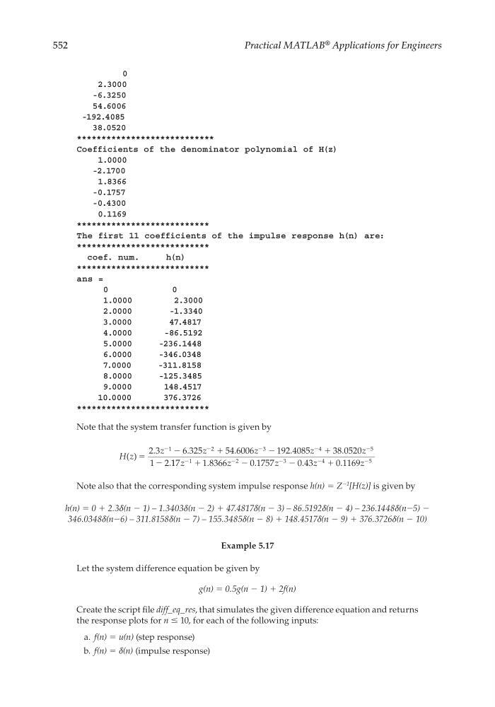
Note that the system transfer function is given by
H z
z
z
z
z
z
( )
.
.
.
.
.
.
ϭ
Ϫ
ϩ
Ϫ
ϩ
Ϫ
Ϫ
Ϫ
Ϫ
Ϫ
Ϫ
2 3
6 325
54 6006
192 4085
38 0520
1 2
1
2
3
4
5
1 17
1 8366
0 1757
0 43
0 1169
1
2
3
4
5
z
z
z
z
z
Ϫ
Ϫ
Ϫ
Ϫ
Ϫ
ϩ
Ϫ
Ϫ
ϩ
.
.
.
.
Note also that the corresponding system impulse response h(n) = Z
−1 [H(z)] is given by
h(n) = 0 + 2.3δ(n − 1) – 1.3403δ(n − 2) + 47.4817δ(n − 3) – 86.5192δ(n − 4) – 236.1448δ(n−5) −
346.0348δ(n−6) – 311.8158δ(n − 7) – 155.3485δ(n − 8) + 148.4517δ(n − 9) + 376.3726δ(n − 10)
Example 5.17
Let the system difference equation be given by
g(n) = 0.5g(n − 1) + 2f(n)
Create the script fi le diff_eq_res, that simulates the given difference equation and returns
the response plots for n ≤ 10, for each of the following inputs:
a. f(n) = u(n) (step response)
b. f(n) = δ(n) (impulse response)
CRC_47760_CH005.indd 552
CRC_47760_CH005.indd 552
7/23/2008 1:47:43 PM
7/23/2008 1:47:43 PM