548
Practical MATLAB
® Applications for Engineers
Error = [part(b)-part(c) versus n
6
8
× 10
−16
4
2
0
−2
−4
−6
−5
0
5
1 0
15
20
25
30
35
time index n
Amplitude
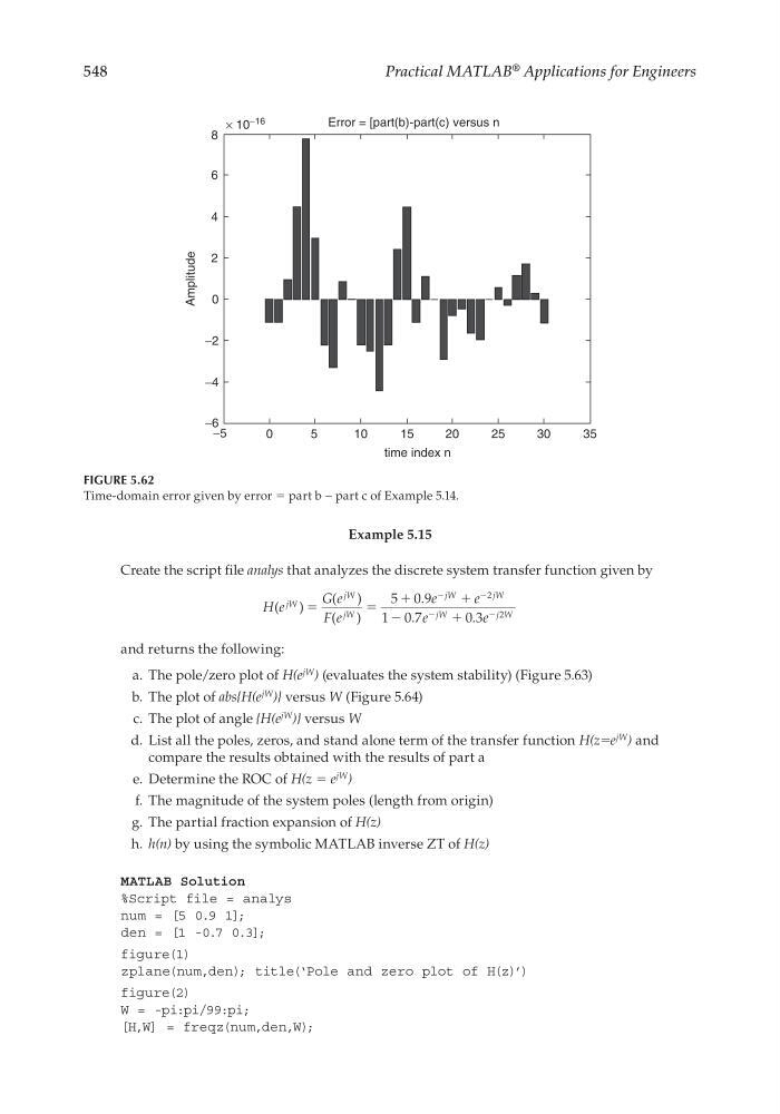
FIGURE 5.62
Time-domain error given by error = part b − part c of Example 5.14.
Example 5.15
Create the script fi le analys that analyzes the discrete system transfer function given by
H e
G e
F e
e
e
e
e
jW
jW
jW
jW
jW
jW
j W
( )
( )
( )
.
.
.
ϭ
ϭ
ϩ
ϩ
Ϫ
ϩ
Ϫ
Ϫ
Ϫ
Ϫ
5 0 9
1 0 7
0 3
2
2
and returns the following:
a. The pole/zero plot of H(e
jW ) (evaluates the system stability) (Figure 5.63)
b. The plot of abs{H(e
jW )} versus W (Figure 5.64)
c. The plot of angle {H(e
jW )} versus W
d. List all the poles, zeros, and stand alone term of the transfer function H(z=e
jW ) and
compare the results obtained with the results of part a
e. Determine the ROC of H(z = e
jW )
f. The magnitude of the system poles (length from origin)
g. The partial fraction expansion of H(z)
h. h(n) by using the symbolic MATLAB inverse ZT of H(z)
MATLAB Solution
%Script file = analys
num = [5 0.9 1];
den = [1 -0.7 0.3];
figure(1)
zplane(num,den); title(‘Pole and zero plot of H(z)’)
figure(2)
W = -pi:pi/99:pi;
[H,W] = freqz(num,den,W);
CRC_47760_CH005.indd 548
CRC_47760_CH005.indd 548
7/23/2008 1:47:42 PM
7/23/2008 1:47:42 PM