DTFT, DFT, ZT, and FFT
541
Example 5.13
The system difference equation of an LTI system is given by
g(n) = 0.7g(n − 1) − 0.3g(n − 2) + f(n) + 0.9f(n − 1)
a. Determine by hand the discrete-transfer function H(z) = G(z)/F(z).
b. Determine by hand H(e
jW ).
c. Obtain the plots of the input f(n) versus n and output g f (n) versus n at steady
state (Figure 5.56), over the range 1 ≤ n ≤ 50, assuming that the input is f(n) =
(0.5)
n sin(0.033πn)u(n), using the MATLAB command fi lter.
d. Obtain the plot of the impulse response h(n) by using the MATLAB command impz
and g(n) by using convolution (Figure 5.57), over the range 1 ≤ n ≤ 50. Let g c (n)
denote the convolution of h(n) with f(n) (time domain) and g f (n) be the system output obtained by the fi lter command (frequency domain).
e. Evaluate and plot the magnitude and phase of fft[g f (n)] and fft[g c (n)], over the range
1 ≤ k ≤ 50 (Figure 5.58).
f. Estimate and plot (Figure 5.59) the error of the above two methods (g f (n) and g c (n))
in the time domain defi ned by the following relation:
error(n) = g f (n) – g c (n), over 1 ≤ n ≤ 50
−2000 −1500
0
0.2
0.4
Magnitude
0.6
0.8
−1000 −500
0
Index n
500
1000 1500
2000
2
1
Phase
0
−1
−2
−3
−2
−1
0
frequency w
1
2
3
× 10 4
error mag.=abs[FT[f(t)]]-abs[DFT[f(n)]] versus w
error phase=angle[FT[f(t)]]-angle[DFT[f(n)]] versus w
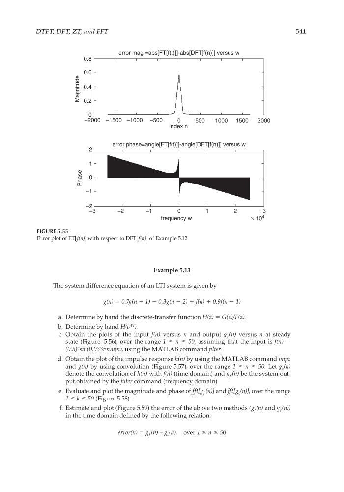
FIGURE 5.55
Error plot of FT[f(n)] with respect to DFT[f(n)] of Example 5.12.
CRC_47760_CH005.indd 541
CRC_47760_CH005.indd 541
7/23/2008 1:47:39 PM
7/23/2008 1:47:39 PM