528
Practical MATLAB
® Applications for Engineers
[Magnitude of the DFTs of f1(n), f2(n) & f3(n)] versus W
0
5
10
15
0
5
10
15
0
5
10
15
0
20
abs [DFT[f3(n)]] abs [DFT[f2(n)]]
abs [DFT[f1(n)]]
40
60
0
0.5
1
1.5
0
10
20
frequency W in rad.
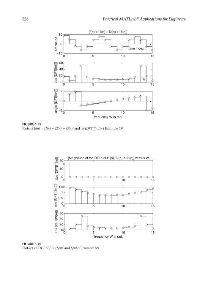
FIGURE 5.40
Plots of absDFT of f 1 (n), f 2 (n), and f 3 (n) of Example 5.9.
[f(n) = f1(n) + f2(n) + f3(n)]
0
0
2
0
20
40
60
−10
0
10
−2
5
1 0
1 5
0
5
10
15
0
5
10
15
frequency W in rad.
angle [DFT[f(n)]]
abs [DFT[f(n)]]
Amplitude
time index n
W
FIGURE 5.39
Plots of [f(n) = f1(n) + f2(n) + f3(n)] and abs{DFT[f(n)]} of Example 5.9.
CRC_47760_CH005.indd 528
CRC_47760_CH005.indd 528
7/23/2008 1:47:35 PM
7/23/2008 1:47:35 PM