

DTFT, DFT, ZT, and FFT
521
Note that the error in the evaluation of g(n) performed by comparing the linear convolution with respect to the circular convolution, is extremely small, in the order of 10
−15
.
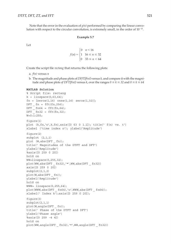
Example 5.7
Let
f n
n
n
n
( ) ϭ
0
16
1 16
32
0 33
64
Ͻ
Յ Յ
Յ Ͻ
Create the script fi le rectang that returns the following plots:
a. f(n) versus n
b. The magnitude and phase plots of DFfT[f(n)] versus k, and compare it with the magnitude and phase plots of DFT[f(n)] versus k, over the ranges 0 ≤ k ≤ 32 and 0 ≤ k ≤ 64
MATLAB Solution
% Script file: rectang
k = linspace(0,63,64);
fn = [zeros(1,16) ones(1,16) zeros(1,32)];
DFT _ fn = fft(fn,256);
DFT _ fn64 = fft(fn,64);
DFT _ fn32 = fft(fn,32);
W=0:1:255;
figure(1)
plot (k,fn,‘o’,k,fn),axis([0 63 0 1.1]); title(‘ f(n) vs. t’)
xlabel (‘time index n’); ylabel(‘Amplitude’)
figure(2)
subplot (2,1,1)
plot (W,abs(DFT _ fn));
title(‘ Magnitudes of the DTFT and DFT’)
ylabel(‘Amplitude’)
%axis([0 259 0 20])
hold on
WW=linspace(0,255,32);
plot(WW,abs(DFT _ fn32),‘*’,WW,abs(DFT _ fn32))
axis([0 259 0 20])
subplot(2,1,2)
plot(W,abs(DFT _ fn));
ylabel(‘Amplitude’)
hold on
WWW= linspace(0,255,64);
plot(WWW,abs(DFT _ fn64),‘o’,WWW,abs(DFT _ fn64));
xlabel(‘ Index k’);axis([0 259 0 20]);
figure(3)
subplot(2,1,1)
plot(W,angle(DFT _ fn));
title(‘ Phase of the DTFT and DFT’)
ylabel(‘Phase angle’)
%axis([0 259 -4 4])
hold on
plot(WW,angle(DFT _ fn32),‘*’,WW,angle(DFT _ fn32))
CRC_47760_CH005.indd 521
CRC_47760_CH005.indd 521
7/23/2008 1:47:34 PM
7/23/2008 1:47:34 PM
521
Note that the error in the evaluation of g(n) performed by comparing the linear convolution with respect to the circular convolution, is extremely small, in the order of 10
−15
.
Example 5.7
Let
f n
n
n
n
( ) ϭ
0
16
1 16
32
0 33
64
Ͻ
Յ Յ
Յ Ͻ
Create the script fi le rectang that returns the following plots:
a. f(n) versus n
b. The magnitude and phase plots of DFfT[f(n)] versus k, and compare it with the magnitude and phase plots of DFT[f(n)] versus k, over the ranges 0 ≤ k ≤ 32 and 0 ≤ k ≤ 64
MATLAB Solution
% Script file: rectang
k = linspace(0,63,64);
fn = [zeros(1,16) ones(1,16) zeros(1,32)];
DFT _ fn = fft(fn,256);
DFT _ fn64 = fft(fn,64);
DFT _ fn32 = fft(fn,32);
W=0:1:255;
figure(1)
plot (k,fn,‘o’,k,fn),axis([0 63 0 1.1]); title(‘ f(n) vs. t’)
xlabel (‘time index n’); ylabel(‘Amplitude’)
figure(2)
subplot (2,1,1)
plot (W,abs(DFT _ fn));
title(‘ Magnitudes of the DTFT and DFT’)
ylabel(‘Amplitude’)
%axis([0 259 0 20])
hold on
WW=linspace(0,255,32);
plot(WW,abs(DFT _ fn32),‘*’,WW,abs(DFT _ fn32))
axis([0 259 0 20])
subplot(2,1,2)
plot(W,abs(DFT _ fn));
ylabel(‘Amplitude’)
hold on
WWW= linspace(0,255,64);
plot(WWW,abs(DFT _ fn64),‘o’,WWW,abs(DFT _ fn64));
xlabel(‘ Index k’);axis([0 259 0 20]);
figure(3)
subplot(2,1,1)
plot(W,angle(DFT _ fn));
title(‘ Phase of the DTFT and DFT’)
ylabel(‘Phase angle’)
%axis([0 259 -4 4])
hold on
plot(WW,angle(DFT _ fn32),‘*’,WW,angle(DFT _ fn32))
CRC_47760_CH005.indd 521
CRC_47760_CH005.indd 521
7/23/2008 1:47:34 PM
7/23/2008 1:47:34 PM