

DTFT, DFT, ZT, and FFT
519
0
1
2
3
4
5
6
7
8
0
1
2
3
4
5
6
7
8
0
1
2
3
4
5
6
7
8
frequency W
frequency W
Phase of DFT[g(n)] versus W
Magnitude of DFT[g(n)] versus W
Linear convolution [g(n) = conv(f(n), h(n))] versus n
time index n
40
100
50
0
20
Amplitude
Magnitude
Angle in rad.
−20
0
5
0
−5
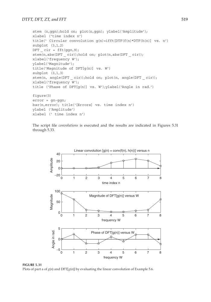
FIGURE 5.31
Plots of part a of g(n) and DFT[g(n)] by evaluating the linear convolution of Example 5.6.
stem (n,ggn);hold on; plot(n,ggn); ylabel(‘Amplitude’);
xlabel (‘time index n’)
title(‘ Circular convolution g(n)=ifft[DTF(f(n)*DTF(h(n)] vs. n’)
subplot (3,1,2)
DFT _ cir = fft(ggn,9);
stem(n,abs(DFT _ cir));hold on; plot(n,abs(DFT _ cir));
xlabel(‘frequency W’);
ylabel(‘Magnitude’);
title(‘Magnitude of DFT[g(n)] vs. W’)
subplot (3,1,3)
stem(n, angle(DFT _ cir));hold on; plot(n, angle(DFT _ cir));
xlabel(‘frequency W’);
title (‘Phase of DFT[g(n)] vs. W’);ylabel(‘Angle in rad.’)
figure(3)
error = gn-ggn;
bar(n,error); title(‘[Errors] vs. time index n’)
ylabel (‘Amplitude’)
xlabel (‘ time index n’)
The script fi le convolutions is executed and the results are indicated in Figures 5.31
through 5.33.
CRC_47760_CH005.indd 519
CRC_47760_CH005.indd 519
7/23/2008 1:47:33 PM
7/23/2008 1:47:33 PM
519
0
1
2
3
4
5
6
7
8
0
1
2
3
4
5
6
7
8
0
1
2
3
4
5
6
7
8
frequency W
frequency W
Phase of DFT[g(n)] versus W
Magnitude of DFT[g(n)] versus W
Linear convolution [g(n) = conv(f(n), h(n))] versus n
time index n
40
100
50
0
20
Amplitude
Magnitude
Angle in rad.
−20
0
5
0
−5
FIGURE 5.31
Plots of part a of g(n) and DFT[g(n)] by evaluating the linear convolution of Example 5.6.
stem (n,ggn);hold on; plot(n,ggn); ylabel(‘Amplitude’);
xlabel (‘time index n’)
title(‘ Circular convolution g(n)=ifft[DTF(f(n)*DTF(h(n)] vs. n’)
subplot (3,1,2)
DFT _ cir = fft(ggn,9);
stem(n,abs(DFT _ cir));hold on; plot(n,abs(DFT _ cir));
xlabel(‘frequency W’);
ylabel(‘Magnitude’);
title(‘Magnitude of DFT[g(n)] vs. W’)
subplot (3,1,3)
stem(n, angle(DFT _ cir));hold on; plot(n, angle(DFT _ cir));
xlabel(‘frequency W’);
title (‘Phase of DFT[g(n)] vs. W’);ylabel(‘Angle in rad.’)
figure(3)
error = gn-ggn;
bar(n,error); title(‘[Errors] vs. time index n’)
ylabel (‘Amplitude’)
xlabel (‘ time index n’)
The script fi le convolutions is executed and the results are indicated in Figures 5.31
through 5.33.
CRC_47760_CH005.indd 519
CRC_47760_CH005.indd 519
7/23/2008 1:47:33 PM
7/23/2008 1:47:33 PM