

Time Domain Representation of Continuous and Discrete Signals
41
R.1.122 For example, let
H Z
z
z
z
z
( )
.
.
.
.
.
ϭ
ϩ
ϩ
ϩ
ϩ
2 24
2 5
2 25
0 5
0 68
2
2
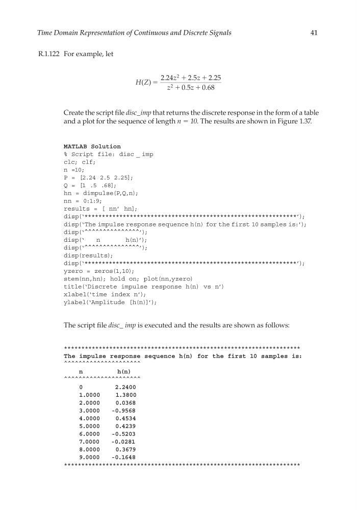
Create the script fi le disc_imp that returns the discrete response in the form of a table
and a plot for the sequence of length n = 10. The results are shown in Figure 1.37.
MATLAB Solution
% Script file: disc _ imp
clc; clf;
n =10;
P = [2.24 2.5 2.25];
Q = [1 .5 .68];
hn = dimpulse(P,Q,n);
nn = 0:1:9;
results = [ nn’ hn];
disp(‘*************************************************************’);
disp(‘The impulse response sequence h(n) for the first 10 samples is:’);
disp(‘^^^^^^^^^^^^^^^’);
disp(‘
n
h(n)’);
disp(‘^^^^^^^^^^^^^^^’);
disp(results);
disp(‘*************************************************************’);
yzero = zeros(1,10);
stem(nn,hn); hold on; plot(nn,yzero)
title(‘Discrete impulse response h(n) vs n’)
xlabel(‘time index n’);
ylabel(‘Amplitude [h(n)]’);
The script fi le disc_ imp is executed and the results are shown as follows:
********************************************************************
The impulse response sequence h(n) for the first 10 samples is:
^^^^^^^^^^^^^^^^^^^^^
n
h(n)
^^^^^^^^^^^^^^^^^^^^^
0
2.2400
1.0000
1.3800
2.0000
0.0368
3.0000
-0.9568
4.0000
0.4534
5.0000
0.4239
6.0000
-0.5203
7.0000
-0.0281
8.0000
0.3679
9.0000
-0.1648
********************************************************************
CRC_47760_CH001.indd 41
CRC_47760_CH001.indd 41
7/25/2008 4:16:18 PM
7/25/2008 4:16:18 PM
41
R.1.122 For example, let
H Z
z
z
z
z
( )
.
.
.
.
.
ϭ
ϩ
ϩ
ϩ
ϩ
2 24
2 5
2 25
0 5
0 68
2
2
Create the script fi le disc_imp that returns the discrete response in the form of a table
and a plot for the sequence of length n = 10. The results are shown in Figure 1.37.
MATLAB Solution
% Script file: disc _ imp
clc; clf;
n =10;
P = [2.24 2.5 2.25];
Q = [1 .5 .68];
hn = dimpulse(P,Q,n);
nn = 0:1:9;
results = [ nn’ hn];
disp(‘*************************************************************’);
disp(‘The impulse response sequence h(n) for the first 10 samples is:’);
disp(‘^^^^^^^^^^^^^^^’);
disp(‘
n
h(n)’);
disp(‘^^^^^^^^^^^^^^^’);
disp(results);
disp(‘*************************************************************’);
yzero = zeros(1,10);
stem(nn,hn); hold on; plot(nn,yzero)
title(‘Discrete impulse response h(n) vs n’)
xlabel(‘time index n’);
ylabel(‘Amplitude [h(n)]’);
The script fi le disc_ imp is executed and the results are shown as follows:
********************************************************************
The impulse response sequence h(n) for the first 10 samples is:
^^^^^^^^^^^^^^^^^^^^^
n
h(n)
^^^^^^^^^^^^^^^^^^^^^
0
2.2400
1.0000
1.3800
2.0000
0.0368
3.0000
-0.9568
4.0000
0.4534
5.0000
0.4239
6.0000
-0.5203
7.0000
-0.0281
8.0000
0.3679
9.0000
-0.1648
********************************************************************
CRC_47760_CH001.indd 41
CRC_47760_CH001.indd 41
7/25/2008 4:16:18 PM
7/25/2008 4:16:18 PM