

508
Practical MATLAB
® Applications for Engineers
Example 5.2
Given the sequences f 1 (n) = [0.3
n u(n)] and f 2 (n) = [0.9
n u(n)]
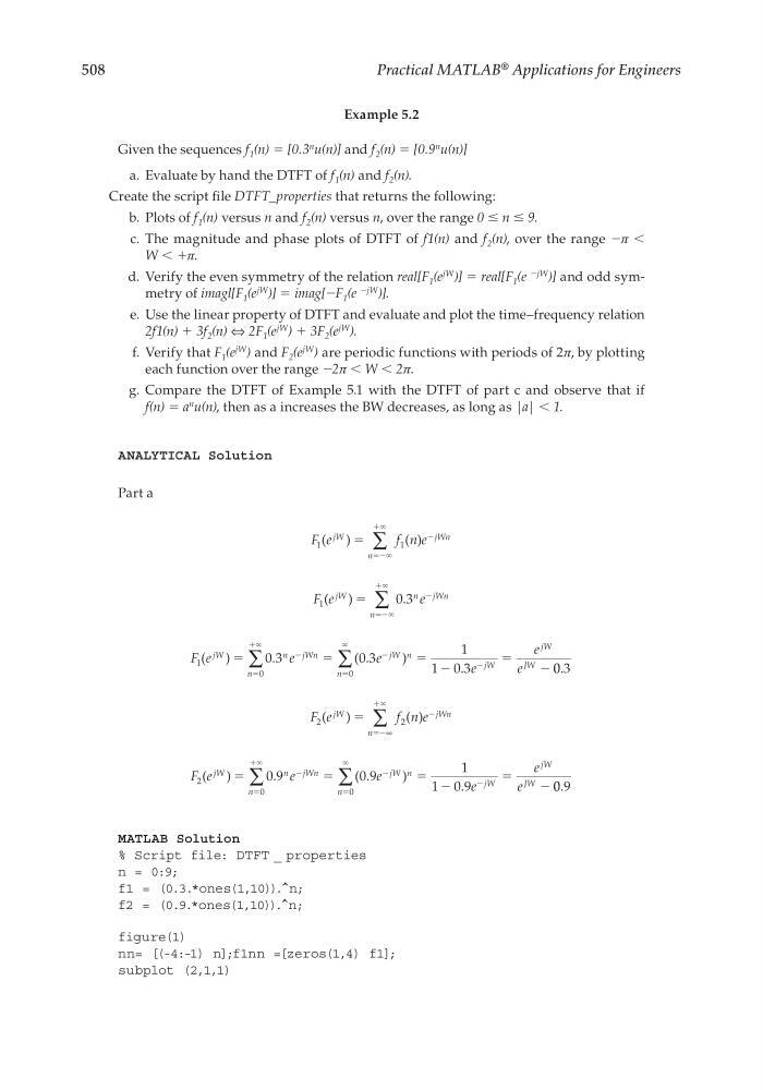
a. Evaluate by hand the DTFT of f 1 (n) and f 2 (n).
Create the script fi le DTFT_properties that returns the following:
b. Plots of f 1 (n) versus n and f 2 (n) versus n, over the range 0 ≤ n ≤ 9.
c. The magnitude and phase plots of DTFT of f1(n) and f 2 (n), over the range −π <
W < +π.
d. Verify the even symmetry of the relation real[F 1 (e
jW )] = real[F 1 (e
−jW )] and odd symmetry of imagl[F 1 (e
jW )] = imag[−F 1 (e
−jW )].
e. Use the linear property of DTFT and evaluate and plot the time–frequency relation
2f1(n) + 3f 2 (n) ⇔ 2F 1 (e
jW ) + 3F 2 (e
jW ).
f. Verify that F 1 (e
jW ) and F 2 (e
jW ) are periodic functions with periods of 2π, by plotting
each function over the range −2π < W < 2π.
g. Compare the DTFT of Example 5.1 with the DTFT of part c and observe that if
f(n) = a
n u(n), then as a increases the BW decreases, as long as |a| < 1.
ANALYTICAL Solution
Part a
F e
f n e
jW
jWn
n
1
1
( )
( )
ϭ
Ϫ
ϭϪϱ
ϩϱ
∑
F e
e
jW
n
jWn
n
1
0 3
( )
.
ϭ
Ϫ
ϭϪϱ
ϩϱ
∑
F e
e
e
e
e
e
jW
n
jWn
n
jW
n
n
jW
jW
JW
1
0
0
0 3
0 3
1
1 0 3
( )
.
( .
)
.
ϭ
ϭ
ϭ Ϫ
ϭ
Ϫ
Ϫ
ϭ
ϩϱ
Ϫ
ϭ
ϱ
Ϫ
∑
∑
0 0 3
.
F e
f n e
jW
jWn
n
2
2
( )
( )
ϭ
Ϫ
ϭϪ
ϩϱ
∞
∑
F e
e
e
e
e
e
jW
n
jWn
n
jW
n
n
jW
jW
JW
2
0
0
0 9
0 9
1
1 0 9
( )
.
( .
)
.
ϭ
ϭ
ϭ Ϫ
ϭ
Ϫ
Ϫ
ϭ
ϩϱ
Ϫ
ϭ
ϱ
Ϫ
∑
∑
0 0 9
.
MATLAB Solution
% Script file: DTFT _ properties
n = 0:9;
f1 = (0.3.*ones(1,10)).^n;
f2 = (0.9.*ones(1,10)).^n;
figure(1)
nn= [(-4:-1) n];f1nn =[zeros(1,4) f1];
subplot (2,1,1)
CRC_47760_CH005.indd 508
CRC_47760_CH005.indd 508
7/23/2008 1:47:30 PM
7/23/2008 1:47:30 PM
Practical MATLAB
® Applications for Engineers
Example 5.2
Given the sequences f 1 (n) = [0.3
n u(n)] and f 2 (n) = [0.9
n u(n)]
a. Evaluate by hand the DTFT of f 1 (n) and f 2 (n).
Create the script fi le DTFT_properties that returns the following:
b. Plots of f 1 (n) versus n and f 2 (n) versus n, over the range 0 ≤ n ≤ 9.
c. The magnitude and phase plots of DTFT of f1(n) and f 2 (n), over the range −π <
W < +π.
d. Verify the even symmetry of the relation real[F 1 (e
jW )] = real[F 1 (e
−jW )] and odd symmetry of imagl[F 1 (e
jW )] = imag[−F 1 (e
−jW )].
e. Use the linear property of DTFT and evaluate and plot the time–frequency relation
2f1(n) + 3f 2 (n) ⇔ 2F 1 (e
jW ) + 3F 2 (e
jW ).
f. Verify that F 1 (e
jW ) and F 2 (e
jW ) are periodic functions with periods of 2π, by plotting
each function over the range −2π < W < 2π.
g. Compare the DTFT of Example 5.1 with the DTFT of part c and observe that if
f(n) = a
n u(n), then as a increases the BW decreases, as long as |a| < 1.
ANALYTICAL Solution
Part a
F e
f n e
jW
jWn
n
1
1
( )
( )
ϭ
Ϫ
ϭϪϱ
ϩϱ
∑
F e
e
jW
n
jWn
n
1
0 3
( )
.
ϭ
Ϫ
ϭϪϱ
ϩϱ
∑
F e
e
e
e
e
e
jW
n
jWn
n
jW
n
n
jW
jW
JW
1
0
0
0 3
0 3
1
1 0 3
( )
.
( .
)
.
ϭ
ϭ
ϭ Ϫ
ϭ
Ϫ
Ϫ
ϭ
ϩϱ
Ϫ
ϭ
ϱ
Ϫ
∑
∑
0 0 3
.
F e
f n e
jW
jWn
n
2
2
( )
( )
ϭ
Ϫ
ϭϪ
ϩϱ
∞
∑
F e
e
e
e
e
e
jW
n
jWn
n
jW
n
n
jW
jW
JW
2
0
0
0 9
0 9
1
1 0 9
( )
.
( .
)
.
ϭ
ϭ
ϭ Ϫ
ϭ
Ϫ
Ϫ
ϭ
ϩϱ
Ϫ
ϭ
ϱ
Ϫ
∑
∑
0 0 9
.
MATLAB Solution
% Script file: DTFT _ properties
n = 0:9;
f1 = (0.3.*ones(1,10)).^n;
f2 = (0.9.*ones(1,10)).^n;
figure(1)
nn= [(-4:-1) n];f1nn =[zeros(1,4) f1];
subplot (2,1,1)
CRC_47760_CH005.indd 508
CRC_47760_CH005.indd 508
7/23/2008 1:47:30 PM
7/23/2008 1:47:30 PM