

506
Practical MATLAB
® Applications for Engineers
−4
−3
−2
−1
0
1
2
3
4
0.5
1
1.5
2
2.5
DTFT [0.6 n u(n)] = 1./(1-0.6*exp(-j.*W))
frequency W in rad.
−4
−3
−2
−1
0
1
2
3
4
frequency W in rad.
Magnitude
−1
−0.5
0
0.5
1
Phase in rad.
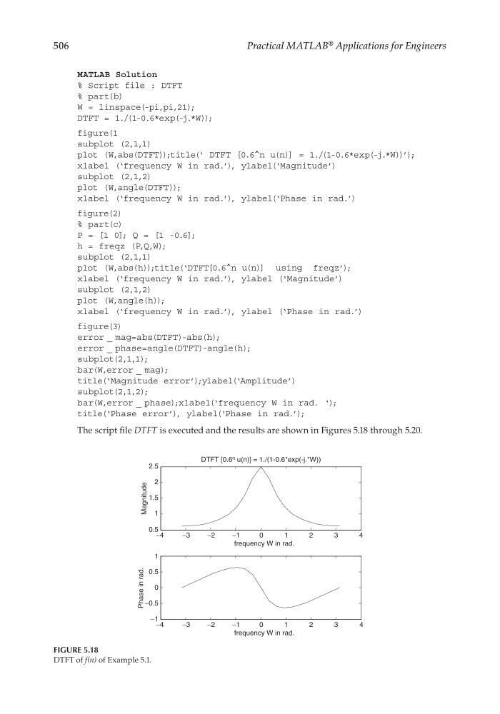
FIGURE 5.18
DTFT of f(n) of Example 5.1.
MATLAB Solution
% Script file : DTFT
% part(b)
W = linspace(-pi,pi,21);
DTFT = 1./(1-0.6*exp(-j.*W));
figure(1
subplot (2,1,1)
plot (W,abs(DTFT));title(‘ DTFT [0.6^n u(n)] = 1./(1-0.6*exp(-j.*W))’);
xlabel (‘frequency W in rad.’), ylabel(‘Magnitude’)
subplot (2,1,2)
plot (W,angle(DTFT));
xlabel (‘frequency W in rad.’), ylabel(‘Phase in rad.’)
figure(2)
% part(c)
P = [1 0]; Q = [1 -0.6];
h = freqz (P,Q,W);
subplot (2,1,1)
plot (W,abs(h));title(‘DTFT[0.6^n u(n)] using freqz’);
xlabel (‘frequency W in rad.’), ylabel (‘Magnitude’)
subplot (2,1,2)
plot (W,angle(h));
xlabel (‘frequency W in rad.’), ylabel (‘Phase in rad.’)
figure(3)
error _ mag=abs(DTFT)-abs(h);
error _ phase=angle(DTFT)-angle(h);
subplot(2,1,1);
bar(W,error _ mag);
title(‘Magnitude error’);ylabel(‘Amplitude’)
subplot(2,1,2);
bar(W,error _ phase);xlabel(‘frequency W in rad. ‘);
title(‘Phase error’), ylabel(‘Phase in rad.’);
The script fi le DTFT is executed and the results are shown in Figures 5.18 through 5.20.
CRC_47760_CH005.indd 506
CRC_47760_CH005.indd 506
7/23/2008 1:47:30 PM
7/23/2008 1:47:30 PM
Practical MATLAB
® Applications for Engineers
−4
−3
−2
−1
0
1
2
3
4
0.5
1
1.5
2
2.5
DTFT [0.6 n u(n)] = 1./(1-0.6*exp(-j.*W))
frequency W in rad.
−4
−3
−2
−1
0
1
2
3
4
frequency W in rad.
Magnitude
−1
−0.5
0
0.5
1
Phase in rad.
FIGURE 5.18
DTFT of f(n) of Example 5.1.
MATLAB Solution
% Script file : DTFT
% part(b)
W = linspace(-pi,pi,21);
DTFT = 1./(1-0.6*exp(-j.*W));
figure(1
subplot (2,1,1)
plot (W,abs(DTFT));title(‘ DTFT [0.6^n u(n)] = 1./(1-0.6*exp(-j.*W))’);
xlabel (‘frequency W in rad.’), ylabel(‘Magnitude’)
subplot (2,1,2)
plot (W,angle(DTFT));
xlabel (‘frequency W in rad.’), ylabel(‘Phase in rad.’)
figure(2)
% part(c)
P = [1 0]; Q = [1 -0.6];
h = freqz (P,Q,W);
subplot (2,1,1)
plot (W,abs(h));title(‘DTFT[0.6^n u(n)] using freqz’);
xlabel (‘frequency W in rad.’), ylabel (‘Magnitude’)
subplot (2,1,2)
plot (W,angle(h));
xlabel (‘frequency W in rad.’), ylabel (‘Phase in rad.’)
figure(3)
error _ mag=abs(DTFT)-abs(h);
error _ phase=angle(DTFT)-angle(h);
subplot(2,1,1);
bar(W,error _ mag);
title(‘Magnitude error’);ylabel(‘Amplitude’)
subplot(2,1,2);
bar(W,error _ phase);xlabel(‘frequency W in rad. ‘);
title(‘Phase error’), ylabel(‘Phase in rad.’);
The script fi le DTFT is executed and the results are shown in Figures 5.18 through 5.20.
CRC_47760_CH005.indd 506
CRC_47760_CH005.indd 506
7/23/2008 1:47:30 PM
7/23/2008 1:47:30 PM