

492
Practical MATLAB
® Applications for Engineers
For the signal f(t) = cos(2πt) just considered (R.5.98), the power spectrum for the
positive frequency range is illustrated as follows:
MATLAB Solution
>> p = abs(fft(fn))/4;
>> power = (p(1:4).^2)’
power =
0.0000
1.0000
0.0000
0.0000
Note that the power content is 1 at the frequency of 1.
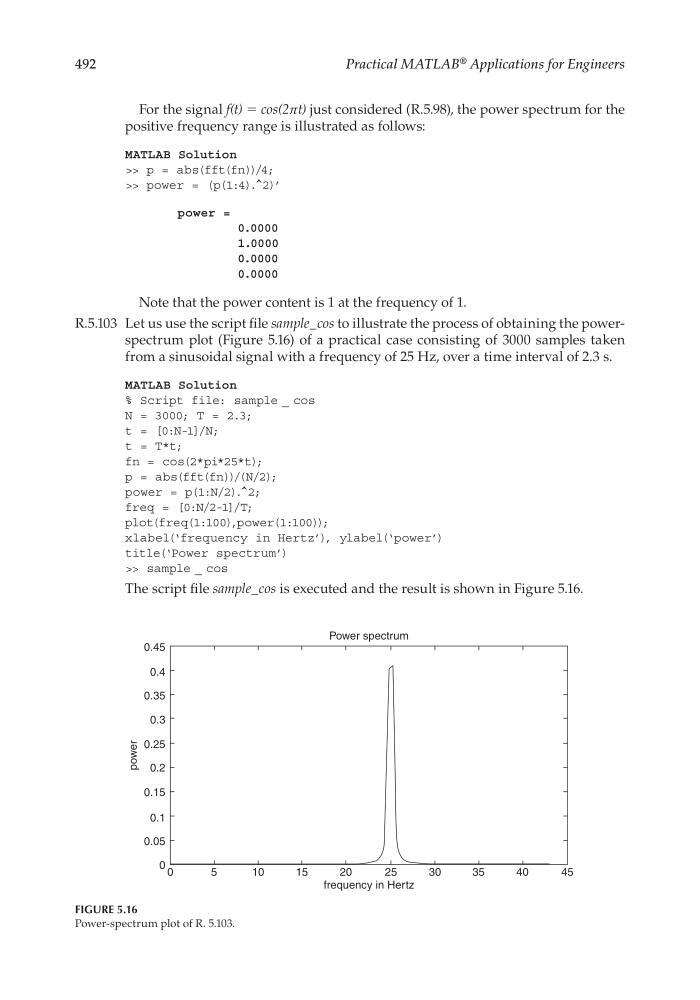
R.5.103 Let us use the script fi le sample_cos to illustrate the process of obtaining the powerspectrum plot (Figure 5.16) of a practical case consisting of 3000 samples taken
from a sinusoidal signal with a frequency of 25 Hz, over a time interval of 2.3 s.
MATLAB Solution
% Script file: sample _ cos
N = 3000; T = 2.3;
t = [0:N-1]/N;
t = T*t;
fn = cos(2*pi*25*t);
p = abs(fft(fn))/(N/2);
power = p(1:N/2).^2;
freq = [0:N/2-1]/T;
plot(freq(1:100),power(1:100));
xlabel(‘frequency in Hertz’), ylabel(‘power’)
title(‘Power spectrum’)
>> sample _ cos
The script fi le sample_cos is executed and the result is shown in Figure 5.16.
25
frequency in Hertz
30
35
40
45
0.45
0.4
0.35
0.3
0.25
power
0.2
0.15
0.1
0.05
0 0
5
10
15
20
Power spectrum
FIGURE 5.16
Power-spectrum plot of R. 5.103.
CRC_47760_CH005.indd 492
CRC_47760_CH005.indd 492
7/23/2008 1:47:26 PM
7/23/2008 1:47:26 PM
Practical MATLAB
® Applications for Engineers
For the signal f(t) = cos(2πt) just considered (R.5.98), the power spectrum for the
positive frequency range is illustrated as follows:
MATLAB Solution
>> p = abs(fft(fn))/4;
>> power = (p(1:4).^2)’
power =
0.0000
1.0000
0.0000
0.0000
Note that the power content is 1 at the frequency of 1.
R.5.103 Let us use the script fi le sample_cos to illustrate the process of obtaining the powerspectrum plot (Figure 5.16) of a practical case consisting of 3000 samples taken
from a sinusoidal signal with a frequency of 25 Hz, over a time interval of 2.3 s.
MATLAB Solution
% Script file: sample _ cos
N = 3000; T = 2.3;
t = [0:N-1]/N;
t = T*t;
fn = cos(2*pi*25*t);
p = abs(fft(fn))/(N/2);
power = p(1:N/2).^2;
freq = [0:N/2-1]/T;
plot(freq(1:100),power(1:100));
xlabel(‘frequency in Hertz’), ylabel(‘power’)
title(‘Power spectrum’)
>> sample _ cos
The script fi le sample_cos is executed and the result is shown in Figure 5.16.
25
frequency in Hertz
30
35
40
45
0.45
0.4
0.35
0.3
0.25
power
0.2
0.15
0.1
0.05
0 0
5
10
15
20
Power spectrum
FIGURE 5.16
Power-spectrum plot of R. 5.103.
CRC_47760_CH005.indd 492
CRC_47760_CH005.indd 492
7/23/2008 1:47:26 PM
7/23/2008 1:47:26 PM