

DTFT, DFT, ZT, and FFT
467
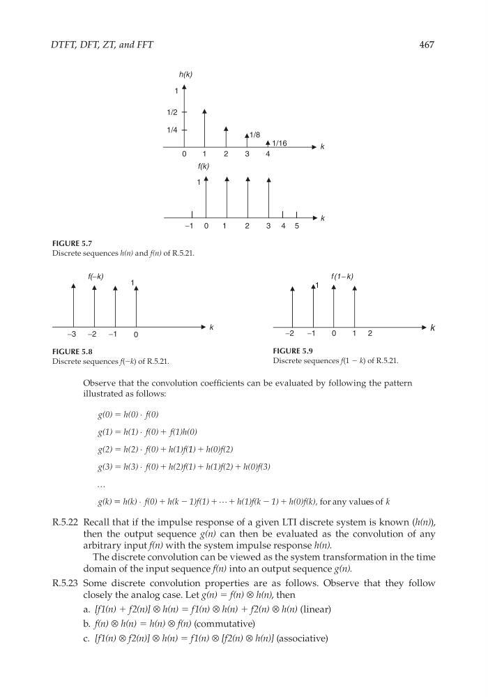
Observe that the convolution coeffi cients can be evaluated by following the pattern
illustrated as follows:
g(0) h(0) f(0)
g(1) h(1) f(0) f(1)h(0)
g(2) h(2) f(0) h(1)f(
ϭ
ϭ
ϩ
ϭ
ϩ
⋅
⋅
⋅
1 1) h(0)f(2)
g(3) h(3) f(0) h(2)f(1) h(1)f(2) h(0)f(3)
g(k)
ϩ
ϭ
ϩ
ϩ
ϩ
⋅
…
ϭ ϭ
ϩ
Ϫ
ϩ ϩ
Ϫ ϩ
h(k) f(0) h(k 1)f(1)
h(1)f(k 1) h(0)f(k),
⋅
for any value es of k
R.5.22 Recall that if the impulse response of a given LTI discrete system is known (h(n)),
then the output sequence g(n) can then be evaluated as the convolution of any
arbitrary input f(n) with the system impulse response h(n).
The discrete convolution can be viewed as the system transformation in the time
domain of the input sequence f(n) into an output sequence g(n).
R.5.23 Some discrete convolution properties are as follows. Observe that they follow
closely the analog case. Let g(n) = f(n) ⊗ h(n), then
a. [f1(n) + f2(n)] ⊗ h(n) = f1(n) ⊗ h(n) + f2(n) ⊗ h(n) (linear)
b. f(n) ⊗ h(n) = h(n) ⊗ f(n) (commutative)
c. [f1(n) ⊗ f2(n)] ⊗ h(n) = f1(n) ⊗ [f2(n) ⊗ h(n)] (associative)
FIGURE 5.7
Discrete sequences h(n) and f(n) of R.5.21.
h(k)
1
1
k
f(k)
k
−1 0
0
1
2
3 4
1
2
3
4
5
1/2
1/4
1/16
1/8
FIGURE 5.8
Discrete sequences f(−k) of R.5.21.
k
−3
−2
−1
1
0
f(−k)
FIGURE 5.9
Discrete sequences f(1 − k) of R.5.21.
1
k
−2
−1
0
1 2
f(1− k)
CRC_47760_CH005.indd 467
CRC_47760_CH005.indd 467
7/23/2008 1:47:18 PM
7/23/2008 1:47:18 PM
467
Observe that the convolution coeffi cients can be evaluated by following the pattern
illustrated as follows:
g(0) h(0) f(0)
g(1) h(1) f(0) f(1)h(0)
g(2) h(2) f(0) h(1)f(
ϭ
ϭ
ϩ
ϭ
ϩ
⋅
⋅
⋅
1 1) h(0)f(2)
g(3) h(3) f(0) h(2)f(1) h(1)f(2) h(0)f(3)
g(k)
ϩ
ϭ
ϩ
ϩ
ϩ
⋅
…
ϭ ϭ
ϩ
Ϫ
ϩ ϩ
Ϫ ϩ
h(k) f(0) h(k 1)f(1)
h(1)f(k 1) h(0)f(k),
⋅
for any value es of k
R.5.22 Recall that if the impulse response of a given LTI discrete system is known (h(n)),
then the output sequence g(n) can then be evaluated as the convolution of any
arbitrary input f(n) with the system impulse response h(n).
The discrete convolution can be viewed as the system transformation in the time
domain of the input sequence f(n) into an output sequence g(n).
R.5.23 Some discrete convolution properties are as follows. Observe that they follow
closely the analog case. Let g(n) = f(n) ⊗ h(n), then
a. [f1(n) + f2(n)] ⊗ h(n) = f1(n) ⊗ h(n) + f2(n) ⊗ h(n) (linear)
b. f(n) ⊗ h(n) = h(n) ⊗ f(n) (commutative)
c. [f1(n) ⊗ f2(n)] ⊗ h(n) = f1(n) ⊗ [f2(n) ⊗ h(n)] (associative)
FIGURE 5.7
Discrete sequences h(n) and f(n) of R.5.21.
h(k)
1
1
k
f(k)
k
−1 0
0
1
2
3 4
1
2
3
4
5
1/2
1/4
1/16
1/8
FIGURE 5.8
Discrete sequences f(−k) of R.5.21.
k
−3
−2
−1
1
0
f(−k)
FIGURE 5.9
Discrete sequences f(1 − k) of R.5.21.
1
k
−2
−1
0
1 2
f(1− k)
CRC_47760_CH005.indd 467
CRC_47760_CH005.indd 467
7/23/2008 1:47:18 PM
7/23/2008 1:47:18 PM