

Fourier and Laplace
451
h(t ) = x (t )
−1.5 0
1.5 t
input x(t )
output y (t )
x (t )
1
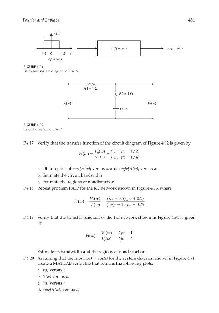
FIGURE 4.91
Block box system diagram of P.4.16.
R1 = 1 Ω
R2 = 1 Ω
C = 2 F
V i (w)
V 0 (w)
FIGURE 4.92
Circuit diagram of P.4.17.
P.4.17 Verify that the transfer function of the circuit diagram of Figure 4.92 is given by
H w
V w
V w
jw
jw
i
( )
( )
( )
(
/ )
(
/ )
ϭ
ϭ
ϩ
ϩ
0
1
2
1 2
1 4
a. Obtain plots of mag[H(w)] versus w and angle[H(w)] versus w
b. Estimate the circuit bandwidth
c. Estimate the regions of nondistortion
P.4.18 Repeat problem P.4.17 for the RC network shown in Figure 4.93, where
H w
V w
V w
jw
jw
jw
jw
i
( )
( )
( )
(
. )(
. )
( )
.
.
ϭ
ϭ
ϩ
ϩ
ϩ
0
2
0 5
0 5
1 5
0 25
ϩ
P.4.19 Verify that the transfer function of the RC network shown in Figure 4.94 is given
by
H w
V w
V w
jw
jw
i
( )
( )
( )
ϭ
ϭ
ϩ
ϩ
0
2
1
2
2
Estimate its bandwidth and the regions of nondistortion.
P.4.20 Assuming that the input x(t) = cos(t) for the system diagram shown in Figure 4.91,
create a MATLAB script fi le that returns the following plots:
a. x(t) versus t
b. X(w) versus w
c. h(t) versus t
d. mag[H(w)] versus w
CRC_47760_CH004.indd 451
CRC_47760_CH004.indd 451
7/28/2008 12:26:24 PM
7/28/2008 12:26:24 PM
451
h(t ) = x (t )
−1.5 0
1.5 t
input x(t )
output y (t )
x (t )
1
FIGURE 4.91
Block box system diagram of P.4.16.
R1 = 1 Ω
R2 = 1 Ω
C = 2 F
V i (w)
V 0 (w)
FIGURE 4.92
Circuit diagram of P.4.17.
P.4.17 Verify that the transfer function of the circuit diagram of Figure 4.92 is given by
H w
V w
V w
jw
jw
i
( )
( )
( )
(
/ )
(
/ )
ϭ
ϭ
ϩ
ϩ
0
1
2
1 2
1 4
a. Obtain plots of mag[H(w)] versus w and angle[H(w)] versus w
b. Estimate the circuit bandwidth
c. Estimate the regions of nondistortion
P.4.18 Repeat problem P.4.17 for the RC network shown in Figure 4.93, where
H w
V w
V w
jw
jw
jw
jw
i
( )
( )
( )
(
. )(
. )
( )
.
.
ϭ
ϭ
ϩ
ϩ
ϩ
0
2
0 5
0 5
1 5
0 25
ϩ
P.4.19 Verify that the transfer function of the RC network shown in Figure 4.94 is given
by
H w
V w
V w
jw
jw
i
( )
( )
( )
ϭ
ϭ
ϩ
ϩ
0
2
1
2
2
Estimate its bandwidth and the regions of nondistortion.
P.4.20 Assuming that the input x(t) = cos(t) for the system diagram shown in Figure 4.91,
create a MATLAB script fi le that returns the following plots:
a. x(t) versus t
b. X(w) versus w
c. h(t) versus t
d. mag[H(w)] versus w
CRC_47760_CH004.indd 451
CRC_47760_CH004.indd 451
7/28/2008 12:26:24 PM
7/28/2008 12:26:24 PM