

Time Domain Representation of Continuous and Discrete Signals
35
Sawtooth(t,.50) versus t
2*Sawtooth(t,.25) versus t
1.5
0.5
0
0
5
1 0
−0.5
−1
−1.5
1
f1(t)
f2(t)
f3(t)
3*Sawtooth(t,.33) versus t
4*Sawtooth(t,.75) versus t
2
1
0
0
5
1 0
−1
−2
5
−5
0
0
5
10
f4(t)
t (time)
4
2
−2
−4
0
0
5
1 0
t (time)
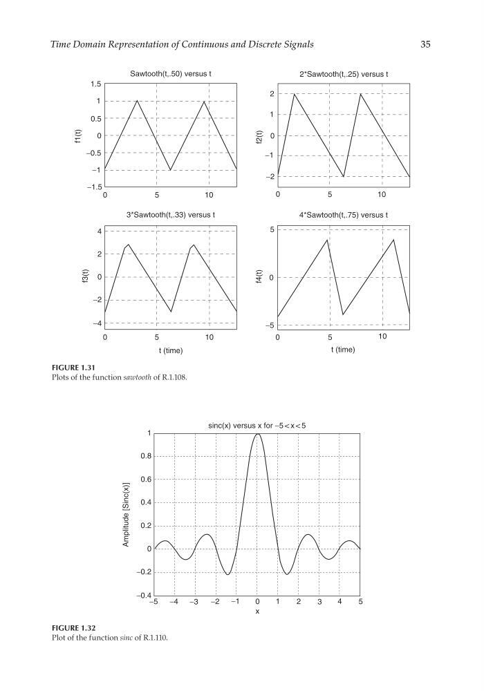
FIGURE 1.31
Plots of the function sawtooth of R.1.108.
FIGURE 1.32
Plot of the function sinc of R.1.110.
sinc(x) versus x for −5 < x < 5
1
0.8
0.6
0.4
0.2
0
−0.2
−0.4
−5
−4 −3
−2
−1
0
1
2
3
4
5
x
Amplitude [Sinc(x)]
CRC_47760_CH001.indd 35
CRC_47760_CH001.indd 35
7/25/2008 4:16:17 PM
7/25/2008 4:16:17 PM
35
Sawtooth(t,.50) versus t
2*Sawtooth(t,.25) versus t
1.5
0.5
0
0
5
1 0
−0.5
−1
−1.5
1
f1(t)
f2(t)
f3(t)
3*Sawtooth(t,.33) versus t
4*Sawtooth(t,.75) versus t
2
1
0
0
5
1 0
−1
−2
5
−5
0
0
5
10
f4(t)
t (time)
4
2
−2
−4
0
0
5
1 0
t (time)
FIGURE 1.31
Plots of the function sawtooth of R.1.108.
FIGURE 1.32
Plot of the function sinc of R.1.110.
sinc(x) versus x for −5 < x < 5
1
0.8
0.6
0.4
0.2
0
−0.2
−0.4
−5
−4 −3
−2
−1
0
1
2
3
4
5
x
Amplitude [Sinc(x)]
CRC_47760_CH001.indd 35
CRC_47760_CH001.indd 35
7/25/2008 4:16:17 PM
7/25/2008 4:16:17 PM