

Fourier and Laplace
419
ANALYTICAL Solution
Recall that
I s
V s
s
s
s
( )
( )
ϭ
ϩ ϩ
⋅ 2 2
10
where the applied voltage is either δ (t) or u(t), with a LT of 1 or 1/s (Table 4.2).
MATLAB Solution
% Script file : repeat _ RLC
num = [0 1 0];
den = [1 2 10];
t = 0:0.1:8*pi;
impres= impulse(num,den,t);
stepres= step(num,den,t);
subplot(2,1,1)
plot(t,impres);title(‘Impulse response ‘);
ylabel(‘magnitude’);axis([0 5 -1 1]);
subplot(2,1,2)
plot(t,stepres);title(‘Step response ‘);
xlabel(‘time(sec)’);ylabel(‘magnitude’);
axis([0 5 -.1 .3])
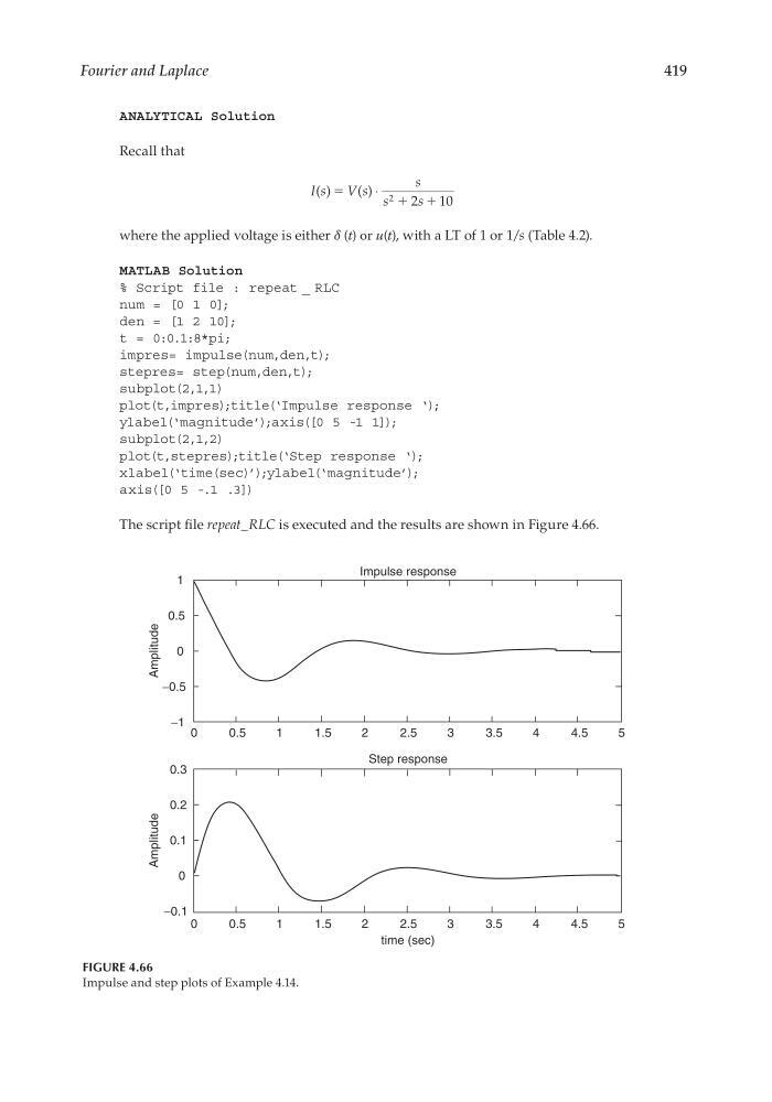
The script fi le repeat_RLC is executed and the results are shown in Figure 4.66.
0
0
0.1
0.2
0.3
1
2
3
4
5
1.5
2.5
3.5
4.5
0.5
0
0
1
1
2
3
4
5
1.5
2.5
3.5
4.5
0.5
0.5
−0.1
−0.5
−1
Amplitude
Amplitude
time (sec)
Step response
Impulse response
FIGURE 4.66
Impulse and step plots of Example 4.14.
CRC_47760_CH004.indd 419
CRC_47760_CH004.indd 419
7/28/2008 12:26:16 PM
7/28/2008 12:26:16 PM
419
ANALYTICAL Solution
Recall that
I s
V s
s
s
s
( )
( )
ϭ
ϩ ϩ
⋅ 2 2
10
where the applied voltage is either δ (t) or u(t), with a LT of 1 or 1/s (Table 4.2).
MATLAB Solution
% Script file : repeat _ RLC
num = [0 1 0];
den = [1 2 10];
t = 0:0.1:8*pi;
impres= impulse(num,den,t);
stepres= step(num,den,t);
subplot(2,1,1)
plot(t,impres);title(‘Impulse response ‘);
ylabel(‘magnitude’);axis([0 5 -1 1]);
subplot(2,1,2)
plot(t,stepres);title(‘Step response ‘);
xlabel(‘time(sec)’);ylabel(‘magnitude’);
axis([0 5 -.1 .3])
The script fi le repeat_RLC is executed and the results are shown in Figure 4.66.
0
0
0.1
0.2
0.3
1
2
3
4
5
1.5
2.5
3.5
4.5
0.5
0
0
1
1
2
3
4
5
1.5
2.5
3.5
4.5
0.5
0.5
−0.1
−0.5
−1
Amplitude
Amplitude
time (sec)
Step response
Impulse response
FIGURE 4.66
Impulse and step plots of Example 4.14.
CRC_47760_CH004.indd 419
CRC_47760_CH004.indd 419
7/28/2008 12:26:16 PM
7/28/2008 12:26:16 PM