

32
Practical MATLAB
® Applications for Engineers
R.1.105 The MATLAB command square(t, a) returns the periodic square wave with period
T = 2 * π, over the range defi ned by t, where a is a constant that indicates the percent of the period T for which the square wave is positive.
R.1.106 For example, create the script fi le squares that returns the plots over two cycles of
the square sequences, with period T = 2π, with the following specs:
a. f 1 (t) versus t, with mag[f 1 (t)] = 1, during 50% of the period T and mag[f 1 (t)] = −1,
during the remaining 50%
b. f 2 (t) versus t, with mag[f 2 (t)] = 2, during 25% of the period T and mag[f 2 (t)] = −2,
during the remaining 75%
c. f 3 (t) versus t, with mag[f 3 (t)] = 3, during 33% of the period T and mag[f 3 (t)] = −3,
during the remaining 67%
d. f 4 (t) versus t, with mag[f 4 (t)] = 4, during 75% of the period T and mag[f 4 (t)] = −4,
during the remaining 25%
MATLAB Solution
% Script file: squares
t = 0:.1*pi:4*pi;
f1 =square(t,50);
f2 =2*square(t,25);
f3 =3*square(t,33);
f4 =4*square(t,75);
subplot(2,2,1)
plot(t,f1)
ylabel(‘f1(t)’)
axis([0 4*pi -1.5 1.5])
grid on;
title(‘Square(t,50) vs t’)
subplot(2,2,2)
plot(t,f2)
heaviside (t)*t versus t
3
2.5
2
1.5
1
0.5
0
−1
−0.5
0
0.5
1
1.5
2
2.5
3
t
t*u(t)
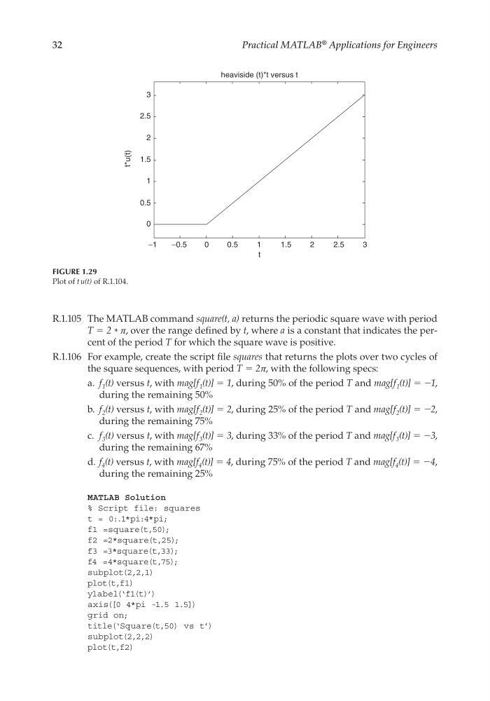
FIGURE 1.29
Plot of t u(t) of R.1.104.
CRC_47760_CH001.indd 32
CRC_47760_CH001.indd 32
7/25/2008 4:16:16 PM
7/25/2008 4:16:16 PM
Practical MATLAB
® Applications for Engineers
R.1.105 The MATLAB command square(t, a) returns the periodic square wave with period
T = 2 * π, over the range defi ned by t, where a is a constant that indicates the percent of the period T for which the square wave is positive.
R.1.106 For example, create the script fi le squares that returns the plots over two cycles of
the square sequences, with period T = 2π, with the following specs:
a. f 1 (t) versus t, with mag[f 1 (t)] = 1, during 50% of the period T and mag[f 1 (t)] = −1,
during the remaining 50%
b. f 2 (t) versus t, with mag[f 2 (t)] = 2, during 25% of the period T and mag[f 2 (t)] = −2,
during the remaining 75%
c. f 3 (t) versus t, with mag[f 3 (t)] = 3, during 33% of the period T and mag[f 3 (t)] = −3,
during the remaining 67%
d. f 4 (t) versus t, with mag[f 4 (t)] = 4, during 75% of the period T and mag[f 4 (t)] = −4,
during the remaining 25%
MATLAB Solution
% Script file: squares
t = 0:.1*pi:4*pi;
f1 =square(t,50);
f2 =2*square(t,25);
f3 =3*square(t,33);
f4 =4*square(t,75);
subplot(2,2,1)
plot(t,f1)
ylabel(‘f1(t)’)
axis([0 4*pi -1.5 1.5])
grid on;
title(‘Square(t,50) vs t’)
subplot(2,2,2)
plot(t,f2)
heaviside (t)*t versus t
3
2.5
2
1.5
1
0.5
0
−1
−0.5
0
0.5
1
1.5
2
2.5
3
t
t*u(t)
FIGURE 1.29
Plot of t u(t) of R.1.104.
CRC_47760_CH001.indd 32
CRC_47760_CH001.indd 32
7/25/2008 4:16:16 PM
7/25/2008 4:16:16 PM