

Fourier and Laplace
417
Y s
Z s
Y s
R sL
sC
s
s
s
s
s
I s
V s
Z
( )
( )
( )
( / )
(
)
( )
( )
ϭ
ϭ ϩ ϩ
ϭ ϩ ϩ
ϭ ϩ
ϩ
ϭ
1
1
1
2
1 0
1
3
2
2
2
( ( )
( ) ( )
s
V s Y s
ϭ
Since
V s
u t
s
( )
[
( )]
ϭ
ϭ
£ 50
50
then
I s
s
s
s
s
i t
I s
e
t
( )
(
)
(
)
( )
[( ( )]
si
ϭ
ϩ
ϩ
ϭ
ϩ
ϩ
ϭ
ϭ
50
1
3
50
3
3
1
3
50
3
2
2
2
2
1
⋅
⋅
£
Ϫ
Ϫ
n n( ) ( )
3t u t
⋅
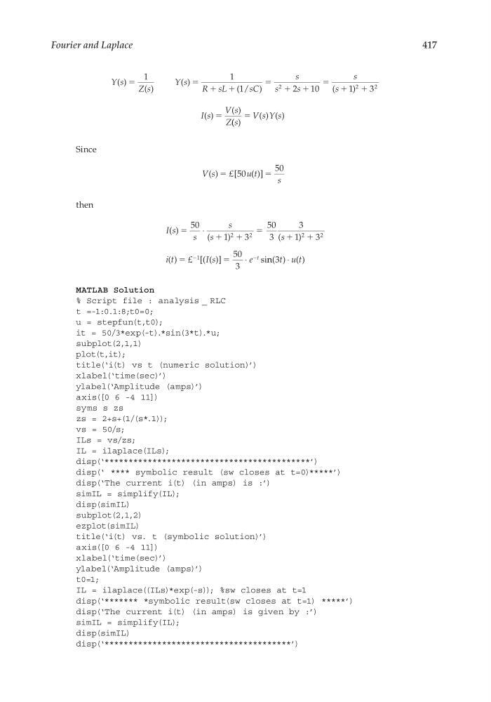
MATLAB Solution
% Script file : analysis _ RLC
t =-1:0.1:8;t0=0;
u = stepfun(t,t0);
it = 50/3*exp(-t).*sin(3*t).*u;
subplot(2,1,1)
plot(t,it);
title(‘i(t) vs t (numeric solution)’)
xlabel(‘time(sec)’)
ylabel(‘Amplitude (amps)’)
axis([0 6 -4 11])
syms s zs
zs = 2+s+(1/(s*.1));
vs = 50/s;
ILs = vs/zs;
IL = ilaplace(ILs);
disp(‘*******************************************’)
disp(‘ **** symbolic result (sw closes at t=0)*****’)
disp(‘The current i(t) (in amps) is :’)
simIL = simplify(IL);
disp(simIL)
subplot(2,1,2)
ezplot(simIL)
title(‘i(t) vs. t (symbolic solution)’)
axis([0 6 -4 11])
xlabel(‘time(sec)’)
ylabel(‘Amplitude (amps)’)
t0=1;
IL = ilaplace((ILs)*exp(-s)); %sw closes at t=1
disp(‘******* *symbolic result(sw closes at t=1) *****’)
disp(‘The current i(t) (in amps) is given by :’)
simIL = simplify(IL);
disp(simIL)
disp(‘***************************************’)
CRC_47760_CH004.indd 417
CRC_47760_CH004.indd 417
7/28/2008 12:26:15 PM
7/28/2008 12:26:15 PM
417
Y s
Z s
Y s
R sL
sC
s
s
s
s
s
I s
V s
Z
( )
( )
( )
( / )
(
)
( )
( )
ϭ
ϭ ϩ ϩ
ϭ ϩ ϩ
ϭ ϩ
ϩ
ϭ
1
1
1
2
1 0
1
3
2
2
2
( ( )
( ) ( )
s
V s Y s
ϭ
Since
V s
u t
s
( )
[
( )]
ϭ
ϭ
£ 50
50
then
I s
s
s
s
s
i t
I s
e
t
( )
(
)
(
)
( )
[( ( )]
si
ϭ
ϩ
ϩ
ϭ
ϩ
ϩ
ϭ
ϭ
50
1
3
50
3
3
1
3
50
3
2
2
2
2
1
⋅
⋅
£
Ϫ
Ϫ
n n( ) ( )
3t u t
⋅
MATLAB Solution
% Script file : analysis _ RLC
t =-1:0.1:8;t0=0;
u = stepfun(t,t0);
it = 50/3*exp(-t).*sin(3*t).*u;
subplot(2,1,1)
plot(t,it);
title(‘i(t) vs t (numeric solution)’)
xlabel(‘time(sec)’)
ylabel(‘Amplitude (amps)’)
axis([0 6 -4 11])
syms s zs
zs = 2+s+(1/(s*.1));
vs = 50/s;
ILs = vs/zs;
IL = ilaplace(ILs);
disp(‘*******************************************’)
disp(‘ **** symbolic result (sw closes at t=0)*****’)
disp(‘The current i(t) (in amps) is :’)
simIL = simplify(IL);
disp(simIL)
subplot(2,1,2)
ezplot(simIL)
title(‘i(t) vs. t (symbolic solution)’)
axis([0 6 -4 11])
xlabel(‘time(sec)’)
ylabel(‘Amplitude (amps)’)
t0=1;
IL = ilaplace((ILs)*exp(-s)); %sw closes at t=1
disp(‘******* *symbolic result(sw closes at t=1) *****’)
disp(‘The current i(t) (in amps) is given by :’)
simIL = simplify(IL);
disp(simIL)
disp(‘***************************************’)
CRC_47760_CH004.indd 417
CRC_47760_CH004.indd 417
7/28/2008 12:26:15 PM
7/28/2008 12:26:15 PM