

404
Practical MATLAB
® Applications for Engineers
ANALYTICAL Solution
Part 1. From Table 4.1, the FT of f(t) = e
−2t u(t) ↔ 1/(jw + 2) (transform # 10).
Part 2. From Table 4.2, the LT of f(t) = e
−2t u(t)↔ 1/(s + 2) (transform # 5).
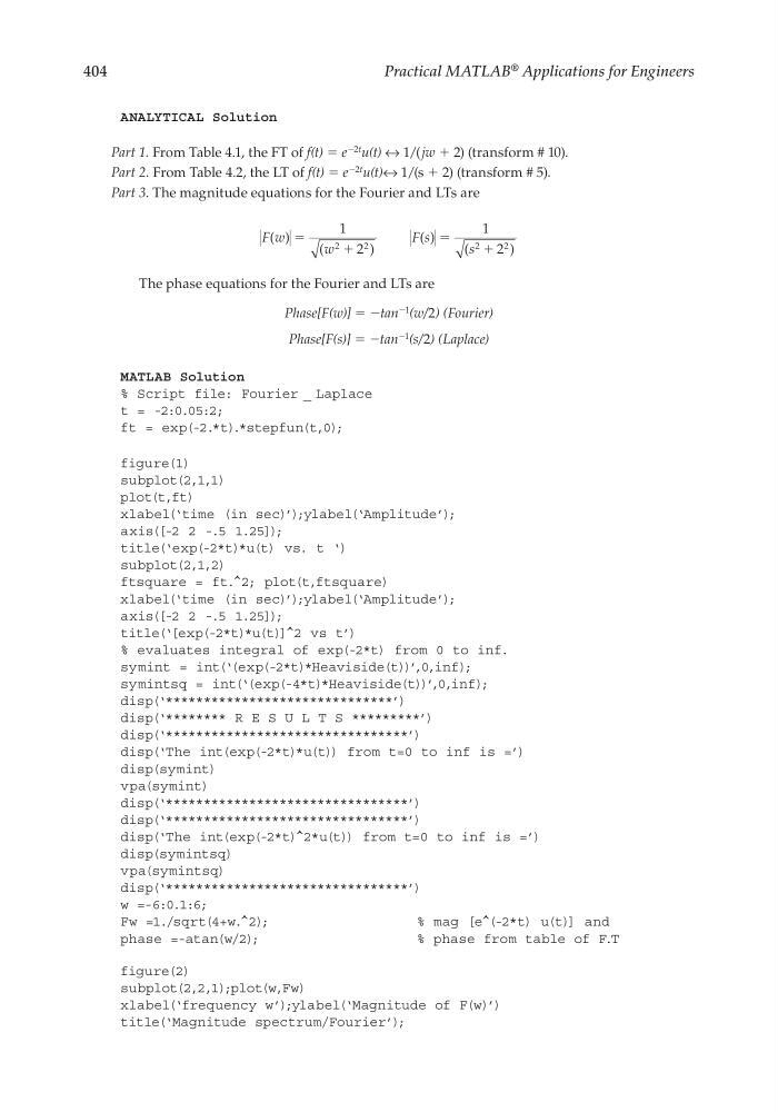
Part 3. The magnitude equations for the Fourier and LTs are
F w
w
F s
s
( )
(
)
( )
(
)
ϭ
ϩ
ϭ
ϩ
1
2
1
2
2
2
2
2
The phase equations for the Fourier and LTs are
Phase[F(w)] = −tan
−1 (w/2) (Fourier)
Phase[F(s)] = −tan
−1 (s/2) (Laplace)
MATLAB Solution
% Script file: Fourier _ Laplace
t = -2:0.05:2;
ft = exp(-2.*t).*stepfun(t,0);
figure(1)
subplot(2,1,1)
plot(t,ft)
xlabel(‘time (in sec)’);ylabel(‘Amplitude’);
axis([-2 2 -.5 1.25]);
title(‘exp(-2*t)*u(t) vs. t ‘)
subplot(2,1,2)
ftsquare = ft.^2; plot(t,ftsquare)
xlabel(‘time (in sec)’);ylabel(‘Amplitude’);
axis([-2 2 -.5 1.25]);
title(‘[exp(-2*t)*u(t)]^2 vs t’)
% evaluates integral of exp(-2*t) from 0 to inf.
symint = int(‘(exp(-2*t)*Heaviside(t))’,0,inf);
symintsq = int(‘(exp(-4*t)*Heaviside(t))’,0,inf);
disp(‘******************************’)
disp(‘******** R E S U L T S *********’)
disp(‘********************************’)
disp(‘The int(exp(-2*t)*u(t)) from t=0 to inf is =’)
disp(symint)
vpa(symint)
disp(‘********************************’)
disp(‘********************************’)
disp(‘The int(exp(-2*t)^2*u(t)) from t=0 to inf is =’)
disp(symintsq)
vpa(symintsq)
disp(‘********************************’)
w =-6:0.1:6;
Fw =1./sqrt(4+w.^2);
% mag [e^(-2*t) u(t)] and
phase =-atan(w/2);
% phase from table of F.T
figure(2)
subplot(2,2,1);plot(w,Fw)
xlabel(‘frequency w’);ylabel(‘Magnitude of F(w)’)
title(‘Magnitude spectrum/Fourier’);
CRC_47760_CH004.indd 404
CRC_47760_CH004.indd 404
7/28/2008 12:26:13 PM
7/28/2008 12:26:13 PM
Practical MATLAB
® Applications for Engineers
ANALYTICAL Solution
Part 1. From Table 4.1, the FT of f(t) = e
−2t u(t) ↔ 1/(jw + 2) (transform # 10).
Part 2. From Table 4.2, the LT of f(t) = e
−2t u(t)↔ 1/(s + 2) (transform # 5).
Part 3. The magnitude equations for the Fourier and LTs are
F w
w
F s
s
( )
(
)
( )
(
)
ϭ
ϩ
ϭ
ϩ
1
2
1
2
2
2
2
2
The phase equations for the Fourier and LTs are
Phase[F(w)] = −tan
−1 (w/2) (Fourier)
Phase[F(s)] = −tan
−1 (s/2) (Laplace)
MATLAB Solution
% Script file: Fourier _ Laplace
t = -2:0.05:2;
ft = exp(-2.*t).*stepfun(t,0);
figure(1)
subplot(2,1,1)
plot(t,ft)
xlabel(‘time (in sec)’);ylabel(‘Amplitude’);
axis([-2 2 -.5 1.25]);
title(‘exp(-2*t)*u(t) vs. t ‘)
subplot(2,1,2)
ftsquare = ft.^2; plot(t,ftsquare)
xlabel(‘time (in sec)’);ylabel(‘Amplitude’);
axis([-2 2 -.5 1.25]);
title(‘[exp(-2*t)*u(t)]^2 vs t’)
% evaluates integral of exp(-2*t) from 0 to inf.
symint = int(‘(exp(-2*t)*Heaviside(t))’,0,inf);
symintsq = int(‘(exp(-4*t)*Heaviside(t))’,0,inf);
disp(‘******************************’)
disp(‘******** R E S U L T S *********’)
disp(‘********************************’)
disp(‘The int(exp(-2*t)*u(t)) from t=0 to inf is =’)
disp(symint)
vpa(symint)
disp(‘********************************’)
disp(‘********************************’)
disp(‘The int(exp(-2*t)^2*u(t)) from t=0 to inf is =’)
disp(symintsq)
vpa(symintsq)
disp(‘********************************’)
w =-6:0.1:6;
Fw =1./sqrt(4+w.^2);
% mag [e^(-2*t) u(t)] and
phase =-atan(w/2);
% phase from table of F.T
figure(2)
subplot(2,2,1);plot(w,Fw)
xlabel(‘frequency w’);ylabel(‘Magnitude of F(w)’)
title(‘Magnitude spectrum/Fourier’);
CRC_47760_CH004.indd 404
CRC_47760_CH004.indd 404
7/28/2008 12:26:13 PM
7/28/2008 12:26:13 PM