

396
Practical MATLAB
® Applications for Engineers
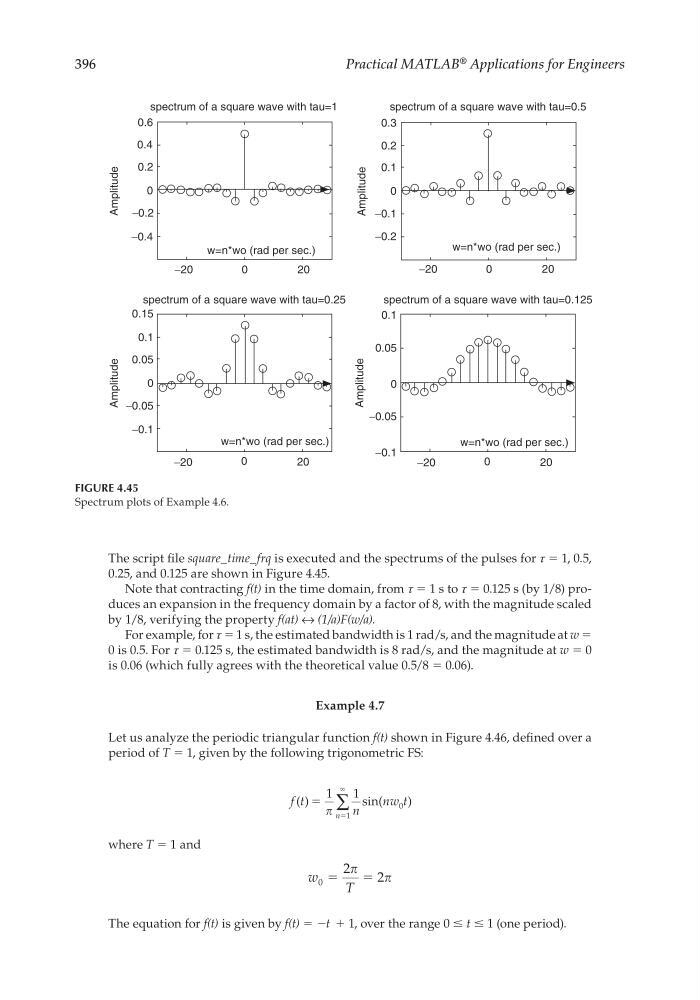
The script fi le square_time_frq is executed and the spectrums of the pulses for τ = 1, 0.5,
0.25, and 0.125 are shown in Figure 4.45.
Note that contracting f(t) in the time domain, from τ = 1 s to τ = 0.125 s (by 1/8) produces an expansion in the frequency domain by a factor of 8, with the magnitude scaled
by 1/8, verifying the property f(at) ↔ (1/a)F(w/a).
For example, for τ = 1 s, the estimated bandwidth is 1 rad/s, and the magnitude at w =
0 is 0.5. For τ = 0.125 s, the estimated bandwidth is 8 rad/s, and the magnitude at w = 0
is 0.06 (which fully agrees with the theoretical value 0.5/8 = 0.06).
Example 4.7
Let us analyze the periodic triangular function f(t) shown in Figure 4.46, defi ned over a
period of T = 1, given by the following trigonometric FS:
f t
n
nw t
n
( )
sin(
)
ϭ
ϭ
1
1
1
0
ϱ
∑
where T = 1 and
w
T
0
2
2
ϭ
ϭ
The equation for f(t) is given by f(t) = −t + 1, over the range 0 ≤ t ≤ 1 (one period).
spectrum of a square wave with tau=1
spectrum of a square wave with tau=0.25
spectrum of a square wave with tau=0.5
spectrum of a square wave with tau=0.125
0.6
0.4
0.2
0
−0.2
−0.4
−20
0
2 0
−20
0
2 0
−20
0
20
−20
0
20
w=n*wo (rad per sec.)
w=n*wo (rad per sec.)
w=n*wo (rad per sec.)
w=n*wo (rad per sec.)
0.3
0.2
0.1
−0.1
−0.2
0
Amplitude
Amplitude
0.1
0.05
0
−0.05
−0.1
0.15
0.1
0.05
−0.05
−0.1
0
Amplitude
Amplitude
FIGURE 4.45
Spectrum plots of Example 4.6.
CRC_47760_CH004.indd 396
CRC_47760_CH004.indd 396
7/28/2008 12:26:11 PM
7/28/2008 12:26:11 PM
Practical MATLAB
® Applications for Engineers
The script fi le square_time_frq is executed and the spectrums of the pulses for τ = 1, 0.5,
0.25, and 0.125 are shown in Figure 4.45.
Note that contracting f(t) in the time domain, from τ = 1 s to τ = 0.125 s (by 1/8) produces an expansion in the frequency domain by a factor of 8, with the magnitude scaled
by 1/8, verifying the property f(at) ↔ (1/a)F(w/a).
For example, for τ = 1 s, the estimated bandwidth is 1 rad/s, and the magnitude at w =
0 is 0.5. For τ = 0.125 s, the estimated bandwidth is 8 rad/s, and the magnitude at w = 0
is 0.06 (which fully agrees with the theoretical value 0.5/8 = 0.06).
Example 4.7
Let us analyze the periodic triangular function f(t) shown in Figure 4.46, defi ned over a
period of T = 1, given by the following trigonometric FS:
f t
n
nw t
n
( )
sin(
)
ϭ
ϭ
1
1
1
0
ϱ
∑
where T = 1 and
w
T
0
2
2
ϭ
ϭ
The equation for f(t) is given by f(t) = −t + 1, over the range 0 ≤ t ≤ 1 (one period).
spectrum of a square wave with tau=1
spectrum of a square wave with tau=0.25
spectrum of a square wave with tau=0.5
spectrum of a square wave with tau=0.125
0.6
0.4
0.2
0
−0.2
−0.4
−20
0
2 0
−20
0
2 0
−20
0
20
−20
0
20
w=n*wo (rad per sec.)
w=n*wo (rad per sec.)
w=n*wo (rad per sec.)
w=n*wo (rad per sec.)
0.3
0.2
0.1
−0.1
−0.2
0
Amplitude
Amplitude
0.1
0.05
0
−0.05
−0.1
0.15
0.1
0.05
−0.05
−0.1
0
Amplitude
Amplitude
FIGURE 4.45
Spectrum plots of Example 4.6.
CRC_47760_CH004.indd 396
CRC_47760_CH004.indd 396
7/28/2008 12:26:11 PM
7/28/2008 12:26:11 PM