

Fourier and Laplace
389
ANALYTICAL Solution
Part 1
f t
F e
n
jnw t
( ) ϭ
Ϫ
ϩ
Ϫ
∞
∞
∑
0
F
e
d t T
w
n
jnw t
ϭ
ϭ
ϭ
1
2
1
2
2
2
0
0 5
0 5
0
( )
;
.
.
Ϫ
Ϫ
ϩ
∫
=
then
F
e
d t
jn
e
n
jnw t
jnw t
ϭ
ϭ
ϩ
1
2
1
1
2
0
0
0 5
0 5
0 5
0 5
( )
.
.
.
.
Ϫ
Ϫ
Ϫ
ϩ
∫
|
F
n
n
n ϭ
1
2
2
2
sin(
)
(
)
ր
ր
Therefore,
f t
n
n
n
( )
sin(
)
(
)
ϭ ϩ
ϭ
ϩ
1
2
1
2
2
2
1
ր
ր
∞
∑
MATLAB Solution
% Script file: Fourier _ series
n = -5:1:5;
% creates harmonics
% add eps to avoid division by zero
Fn = 0.5*sin(n.*pi/2)./((n.*pi/2)+eps);
% creates the coefficients Fn
t =linspace (-2,2,50);
% limits from -1 to 1,one
period
F1=Fn(5)*exp(j*pi.*t)+Fn(7)*exp (-j*pi.*t);
% first component
F2=Fn(4)*exp(j*2*pi.*t)+Fn(8)*exp (-j*2*pi.*t);
% second component
F3=Fn(3)*exp(j*3*pi.*t)+Fn(9)*exp (-j*3*pi.*t);
% third component
F4=Fn(2)*exp(j*4*pi.*t)+Fn(10)*exp (-j*4*pi.*t);
% fourth component
F5=Fn(1)*exp(j*5*pi.*t)+Fn(11)*exp (-j*5*pi.*t);
% fifth component
figure(1);
% see Figure 4.40; part (2a)
F0 = .5.*ones(1,50);
subplot (3,2,1);plot (t,F0);
title (‘DC component’); ylabel (‘Amplitude (F0)’)
subplot (3,2,2);plot (t,F1);
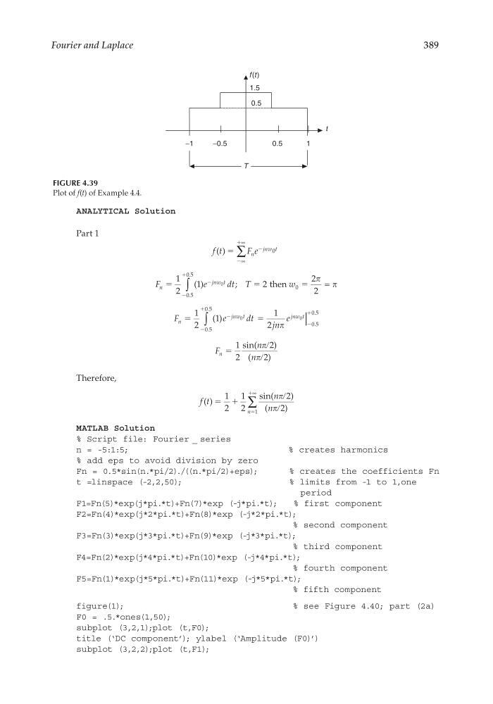
FIGURE 4.39
Plot of f(t) of Example 4.4.
f (t )
1.5
−0.5
0.5
0.5
−1
1
T
t
CRC_47760_CH004.indd 389
CRC_47760_CH004.indd 389
7/28/2008 12:26:09 PM
7/28/2008 12:26:09 PM
389
ANALYTICAL Solution
Part 1
f t
F e
n
jnw t
( ) ϭ
Ϫ
ϩ
Ϫ
∞
∞
∑
0
F
e
d t T
w
n
jnw t
ϭ
ϭ
ϭ
1
2
1
2
2
2
0
0 5
0 5
0
( )
;
.
.
Ϫ
Ϫ
ϩ
∫
=
then
F
e
d t
jn
e
n
jnw t
jnw t
ϭ
ϭ
ϩ
1
2
1
1
2
0
0
0 5
0 5
0 5
0 5
( )
.
.
.
.
Ϫ
Ϫ
Ϫ
ϩ
∫
|
F
n
n
n ϭ
1
2
2
2
sin(
)
(
)
ր
ր
Therefore,
f t
n
n
n
( )
sin(
)
(
)
ϭ ϩ
ϭ
ϩ
1
2
1
2
2
2
1
ր
ր
∞
∑
MATLAB Solution
% Script file: Fourier _ series
n = -5:1:5;
% creates harmonics
% add eps to avoid division by zero
Fn = 0.5*sin(n.*pi/2)./((n.*pi/2)+eps);
% creates the coefficients Fn
t =linspace (-2,2,50);
% limits from -1 to 1,one
period
F1=Fn(5)*exp(j*pi.*t)+Fn(7)*exp (-j*pi.*t);
% first component
F2=Fn(4)*exp(j*2*pi.*t)+Fn(8)*exp (-j*2*pi.*t);
% second component
F3=Fn(3)*exp(j*3*pi.*t)+Fn(9)*exp (-j*3*pi.*t);
% third component
F4=Fn(2)*exp(j*4*pi.*t)+Fn(10)*exp (-j*4*pi.*t);
% fourth component
F5=Fn(1)*exp(j*5*pi.*t)+Fn(11)*exp (-j*5*pi.*t);
% fifth component
figure(1);
% see Figure 4.40; part (2a)
F0 = .5.*ones(1,50);
subplot (3,2,1);plot (t,F0);
title (‘DC component’); ylabel (‘Amplitude (F0)’)
subplot (3,2,2);plot (t,F1);
FIGURE 4.39
Plot of f(t) of Example 4.4.
f (t )
1.5
−0.5
0.5
0.5
−1
1
T
t
CRC_47760_CH004.indd 389
CRC_47760_CH004.indd 389
7/28/2008 12:26:09 PM
7/28/2008 12:26:09 PM