

386
Practical MATLAB
® Applications for Engineers
Example 4.3
Let the FS expansion for a periodic sawtooth wave be given by
f t
( ) ϭ
ϭ
Ϫ1
1
1
6
0
n
nw t
n
∑ sin( ) (same as in Example 4.2)
with period T = 2 s, and fundamental frequency given by w 0 = 2π/T = π.
Let f(t) represent the voltage drop across a resistor R = 5 Ω. Create the script fi le
Fourier_applic that returns the following:
1. The fi rst 10 FS coeffi cients
2. Its RMS value
3. The percentage of the total harmonic distortion
4. The average power dissipated by R = 5 Ω
5. The power concentrated in the fi rst 10 harmonics
6. The plot of the percentage of total power (dissipated) versus its harmonic
frequencies
7. Check the % of total power dissipated in the fi rst 10 harmonics.
MATLAB Solution
% Script file: Fourier _ applic
% Calculations of the Fourier coefficient
for n = 1:10;
c(n) = -1/(n*pi);
p(n) = c(n).^2;
end
C = c;
% RMS calculations
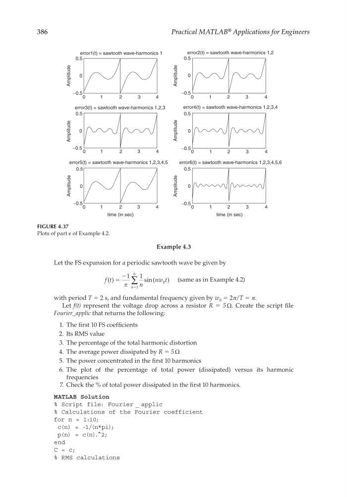
FIGURE 4.37
Plots of part e of Example 4.2.
error1(t) = sawtooth wave-harmonics 1
error3(t) = sawtooth wave-harmonics 1,2,3
error5(t) = sawtooth wave-harmonics 1,2,3,4,5
error2(t) = sawtooth wave-harmonics 1,2
error4(t) = sawtooth wave-harmonics 1,2,3,4
error6(t) = sawtooth wave-harmonics 1,2,3,4,5,6
0.5
0.5
−0.5
−0.5
0
0
0.5
−0.5
0
0.5
−0.5
0
0.5
−0.5
0
0.5
−0.5
0
Amplitude
Amplitude
Amplitude
Amplitude
Amplitude
Amplitude
0
1
2
3
4
0
1
2
3
4
0
1
2
3
4
time (in sec)
time (in sec)
0
1
2
3
4
0
1
2
3
4
0
1
2
3
4
CRC_47760_CH004.indd 386
CRC_47760_CH004.indd 386
7/28/2008 12:26:09 PM
7/28/2008 12:26:09 PM
Practical MATLAB
® Applications for Engineers
Example 4.3
Let the FS expansion for a periodic sawtooth wave be given by
f t
( ) ϭ
ϭ
Ϫ1
1
1
6
0
n
nw t
n
∑ sin( ) (same as in Example 4.2)
with period T = 2 s, and fundamental frequency given by w 0 = 2π/T = π.
Let f(t) represent the voltage drop across a resistor R = 5 Ω. Create the script fi le
Fourier_applic that returns the following:
1. The fi rst 10 FS coeffi cients
2. Its RMS value
3. The percentage of the total harmonic distortion
4. The average power dissipated by R = 5 Ω
5. The power concentrated in the fi rst 10 harmonics
6. The plot of the percentage of total power (dissipated) versus its harmonic
frequencies
7. Check the % of total power dissipated in the fi rst 10 harmonics.
MATLAB Solution
% Script file: Fourier _ applic
% Calculations of the Fourier coefficient
for n = 1:10;
c(n) = -1/(n*pi);
p(n) = c(n).^2;
end
C = c;
% RMS calculations
FIGURE 4.37
Plots of part e of Example 4.2.
error1(t) = sawtooth wave-harmonics 1
error3(t) = sawtooth wave-harmonics 1,2,3
error5(t) = sawtooth wave-harmonics 1,2,3,4,5
error2(t) = sawtooth wave-harmonics 1,2
error4(t) = sawtooth wave-harmonics 1,2,3,4
error6(t) = sawtooth wave-harmonics 1,2,3,4,5,6
0.5
0.5
−0.5
−0.5
0
0
0.5
−0.5
0
0.5
−0.5
0
0.5
−0.5
0
0.5
−0.5
0
Amplitude
Amplitude
Amplitude
Amplitude
Amplitude
Amplitude
0
1
2
3
4
0
1
2
3
4
0
1
2
3
4
time (in sec)
time (in sec)
0
1
2
3
4
0
1
2
3
4
0
1
2
3
4
CRC_47760_CH004.indd 386
CRC_47760_CH004.indd 386
7/28/2008 12:26:09 PM
7/28/2008 12:26:09 PM