

Fourier and Laplace
367
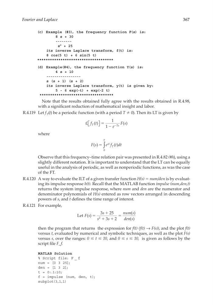
(c) Example (#3), the frequency function F(s) is:
8 s + 30
-------s
2 + 25
its inverse Laplace transform, f(t) is:
8 cos(5 t) + 6 sin(5 t)
************************************
(d) Example(#4), the frequency function Y(s) is:
4 s + 10
----------------s (s + 1) (s + 2)
its inverse Laplace transform, y(t) is given by:
5 - 6 exp(-t) + exp(-2 t)
***********************************
Note that the results obtained fully agree with the results obtained in R.4.98,
with a signifi cant reduction of mathematical insight and labor.
R.4.119 Let f T (t) be a periodic function (with a period T ≠ 0). Then its LT is given by
£ f t
e
F s
T
Ts
( )
( )
ϭ
1
1 Ϫ
Ϫ
where
F s
e f t dt
st
T
T
( )
( )
ϭ
0
∫
Observe that this frequency–time relation pair was presented in R.4.82 (#h), using a
slightly different notation. It is important to understand that the LT can be equally
useful in the analysis of periodic, as well as nonperiodic functions, as was the case
of the FT.
R.4.120 A way to evaluate the ILT of a given transfer function H(s) = num/den is by evaluating its impulse response h(t). Recall that the MATLAB function impulse (num,den,t)
returns the system impulse response, where num and den are the numerator and
denominator polynomials of H(s) entered as row vectors arranged in descending
powers of s, and t defi nes the time range of interest.
R.4.121 For example,
Let F s
s
s
s
s
s
( )
( )
( )
ϭ
ϩ
ϩ ϩ
ϭ
3
25
3
2
2
num
den
then the program that returns the expression for f(t) (f(t) → F(s)), and the plot f(t)
versus t, evaluated by numerical and symbolic techniques, as well as the plot F(s)
versus s, over the ranges: 0 ≤ t ≤ 10, and 0 ≤ s ≤ 10, is given as follows by the
script fi le F_f.
MATLAB Solution
% Script file: F _ f
num = [0 3 25];
den = [1 3 2];
t = 0:.1:10;
f = impulse (num, den, t);
subplot(3,1,1)
CRC_47760_CH004.indd 367
CRC_47760_CH004.indd 367
7/28/2008 12:26:04 PM
7/28/2008 12:26:04 PM
367
(c) Example (#3), the frequency function F(s) is:
8 s + 30
-------s
2 + 25
its inverse Laplace transform, f(t) is:
8 cos(5 t) + 6 sin(5 t)
************************************
(d) Example(#4), the frequency function Y(s) is:
4 s + 10
----------------s (s + 1) (s + 2)
its inverse Laplace transform, y(t) is given by:
5 - 6 exp(-t) + exp(-2 t)
***********************************
Note that the results obtained fully agree with the results obtained in R.4.98,
with a signifi cant reduction of mathematical insight and labor.
R.4.119 Let f T (t) be a periodic function (with a period T ≠ 0). Then its LT is given by
£ f t
e
F s
T
Ts
( )
( )
ϭ
1
1 Ϫ
Ϫ
where
F s
e f t dt
st
T
T
( )
( )
ϭ
0
∫
Observe that this frequency–time relation pair was presented in R.4.82 (#h), using a
slightly different notation. It is important to understand that the LT can be equally
useful in the analysis of periodic, as well as nonperiodic functions, as was the case
of the FT.
R.4.120 A way to evaluate the ILT of a given transfer function H(s) = num/den is by evaluating its impulse response h(t). Recall that the MATLAB function impulse (num,den,t)
returns the system impulse response, where num and den are the numerator and
denominator polynomials of H(s) entered as row vectors arranged in descending
powers of s, and t defi nes the time range of interest.
R.4.121 For example,
Let F s
s
s
s
s
s
( )
( )
( )
ϭ
ϩ
ϩ ϩ
ϭ
3
25
3
2
2
num
den
then the program that returns the expression for f(t) (f(t) → F(s)), and the plot f(t)
versus t, evaluated by numerical and symbolic techniques, as well as the plot F(s)
versus s, over the ranges: 0 ≤ t ≤ 10, and 0 ≤ s ≤ 10, is given as follows by the
script fi le F_f.
MATLAB Solution
% Script file: F _ f
num = [0 3 25];
den = [1 3 2];
t = 0:.1:10;
f = impulse (num, den, t);
subplot(3,1,1)
CRC_47760_CH004.indd 367
CRC_47760_CH004.indd 367
7/28/2008 12:26:04 PM
7/28/2008 12:26:04 PM