

362
Practical MATLAB
® Applications for Engineers
Y s s
( )[
]
2
4
8
Ϫ ϭ
Y s
s
s
( ) ϭ
ϭ
8
4
4
2
2
2
2
2
Ϫ
Ϫ
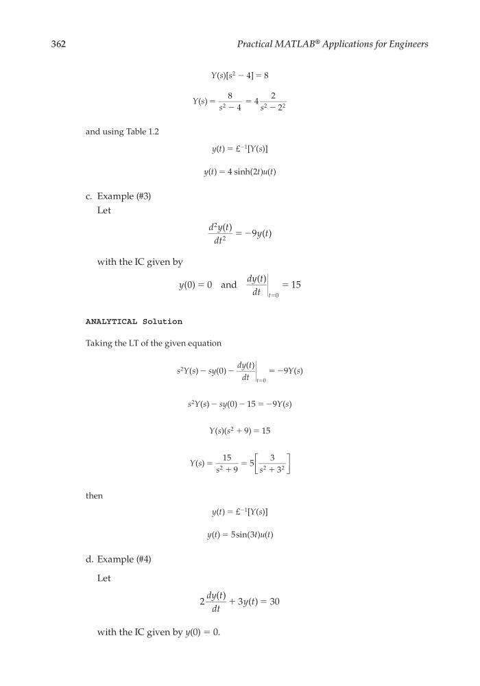
and using Table 1.2
y t
Y s
( )
[ ( )]
ϭ £
Ϫ1
y t
t u t
( )
sinh( ) ( )
ϭ 4
2
c. Example (#3)
Let
d y t
dt
y t
2
2
9
( )
( )
ϭ Ϫ
with the IC given by
y
dy t
dt t
( )
( )
0
0
15
0
ϭ
ϭ
ϭ
and
ANALYTICAL Solution
Taking the LT of the given equation
s Y s
sy
dy t
dt
Y s
t
2
0
0
9
( )
( )
( )
( )
Ϫ
Ϫ
Ϫ
ϭ
ϭ
s Y s
sy
Y s
2
0 15
9
( )
( )
( )
Ϫ
Ϫ
Ϫ
ϭ
Y s s
( )(
)
2
9
15
ϩ ϭ
Y s
s
s
( ) ϭ ϩ
ϭ
ϩ
15
9
5
3
3
2
2
2
then
y t
Y s
( )
[ ( )]
ϭ £
Ϫ1
y t
t u t
( )
sin( ) ( )
ϭ 5
3
d. Example (#4)
Let
2
3
3 0
dy t
dt
y t
( )
( )
ϩ
ϭ
with the IC given by y(0) = 0.
CRC_47760_CH004.indd 362
CRC_47760_CH004.indd 362
7/28/2008 12:26:03 PM
7/28/2008 12:26:03 PM
Practical MATLAB
® Applications for Engineers
Y s s
( )[
]
2
4
8
Ϫ ϭ
Y s
s
s
( ) ϭ
ϭ
8
4
4
2
2
2
2
2
Ϫ
Ϫ
and using Table 1.2
y t
Y s
( )
[ ( )]
ϭ £
Ϫ1
y t
t u t
( )
sinh( ) ( )
ϭ 4
2
c. Example (#3)
Let
d y t
dt
y t
2
2
9
( )
( )
ϭ Ϫ
with the IC given by
y
dy t
dt t
( )
( )
0
0
15
0
ϭ
ϭ
ϭ
and
ANALYTICAL Solution
Taking the LT of the given equation
s Y s
sy
dy t
dt
Y s
t
2
0
0
9
( )
( )
( )
( )
Ϫ
Ϫ
Ϫ
ϭ
ϭ
s Y s
sy
Y s
2
0 15
9
( )
( )
( )
Ϫ
Ϫ
Ϫ
ϭ
Y s s
( )(
)
2
9
15
ϩ ϭ
Y s
s
s
( ) ϭ ϩ
ϭ
ϩ
15
9
5
3
3
2
2
2
then
y t
Y s
( )
[ ( )]
ϭ £
Ϫ1
y t
t u t
( )
sin( ) ( )
ϭ 5
3
d. Example (#4)
Let
2
3
3 0
dy t
dt
y t
( )
( )
ϩ
ϭ
with the IC given by y(0) = 0.
CRC_47760_CH004.indd 362
CRC_47760_CH004.indd 362
7/28/2008 12:26:03 PM
7/28/2008 12:26:03 PM