

24
Practical MATLAB
® Applications for Engineers
ANALYTICAL Solution
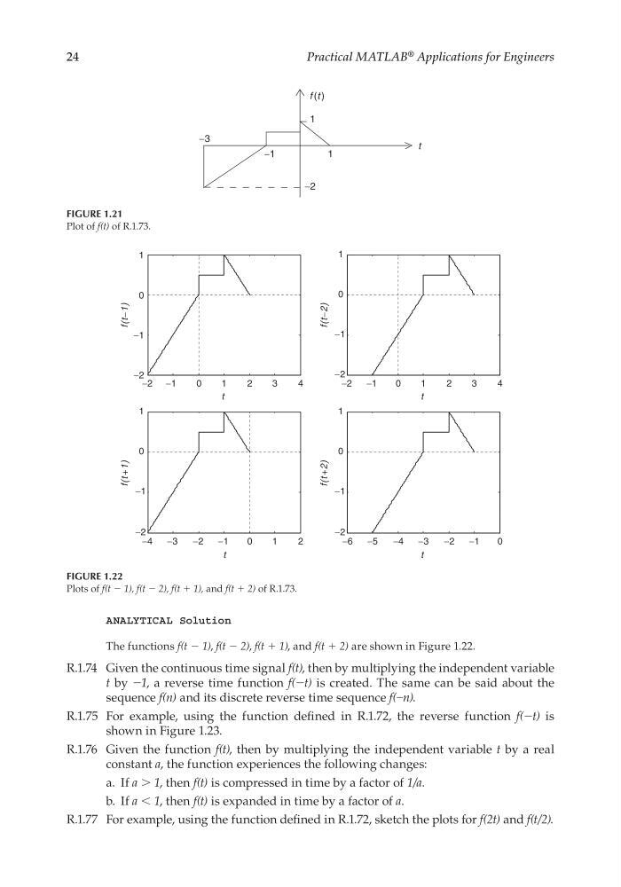
The functions f(t − 1), f(t − 2), f(t + 1), and f(t + 2) are shown in Figure 1.22.
R.1.74 Given the continuous time signal f(t), then by multiplying the independent variable
t by −1, a reverse time function f(−t) is created. The same can be said about the
sequence f(n) and its discrete reverse time sequence f(–n).
R.1.75 For example, using the function defi ned in R.1.72, the reverse function f(−t) is
shown in Figure 1.23.
R.1.76 Given the function f(t), then by multiplying the independent variable t by a real
constant a, the function experiences the following changes:
a. If a > 1, then f(t) is compressed in time by a factor of 1/a.
b. If a < 1, then f(t) is expanded in time by a factor of a.
R.1.77 For example, using the function defi ned in R.1.72, sketch the plots for f(2t) and f(t/2).
−2 −1
0
1
2
3
4
−2
−1
0
1
f(t−1)
t
−2
−1
0
1
2
3
4
−2
−1
0
1
f(t−2)
t
−4
−3
−2
−1
0
1
2
−2
−1
0
1
f(t +1)
t
−6
−5
−4
−3
−2
−1
0
−2
−1
0
1
f(t +2)
t
FIGURE 1.22
Plots of f(t − 1), f(t − 2), f(t + 1), and f(t + 2) of R.1.73.
f (t )
1
1
−1
−2
−3
t
FIGURE 1.21
Plot of f(t) of R.1.73.
CRC_47760_CH001.indd 24
CRC_47760_CH001.indd 24
7/25/2008 4:16:15 PM
7/25/2008 4:16:15 PM
Practical MATLAB
® Applications for Engineers
ANALYTICAL Solution
The functions f(t − 1), f(t − 2), f(t + 1), and f(t + 2) are shown in Figure 1.22.
R.1.74 Given the continuous time signal f(t), then by multiplying the independent variable
t by −1, a reverse time function f(−t) is created. The same can be said about the
sequence f(n) and its discrete reverse time sequence f(–n).
R.1.75 For example, using the function defi ned in R.1.72, the reverse function f(−t) is
shown in Figure 1.23.
R.1.76 Given the function f(t), then by multiplying the independent variable t by a real
constant a, the function experiences the following changes:
a. If a > 1, then f(t) is compressed in time by a factor of 1/a.
b. If a < 1, then f(t) is expanded in time by a factor of a.
R.1.77 For example, using the function defi ned in R.1.72, sketch the plots for f(2t) and f(t/2).
−2 −1
0
1
2
3
4
−2
−1
0
1
f(t−1)
t
−2
−1
0
1
2
3
4
−2
−1
0
1
f(t−2)
t
−4
−3
−2
−1
0
1
2
−2
−1
0
1
f(t +1)
t
−6
−5
−4
−3
−2
−1
0
−2
−1
0
1
f(t +2)
t
FIGURE 1.22
Plots of f(t − 1), f(t − 2), f(t + 1), and f(t + 2) of R.1.73.
f (t )
1
1
−1
−2
−3
t
FIGURE 1.21
Plot of f(t) of R.1.73.
CRC_47760_CH001.indd 24
CRC_47760_CH001.indd 24
7/25/2008 4:16:15 PM
7/25/2008 4:16:15 PM