

328
Practical MATLAB
® Applications for Engineers
b. If f(t) = −f(−t), indicating that f(t) is an odd function with respect to t, then
f t
b
nw t
n
( )
(
)
ϭ
sin
0
n
∑
where
b
T
f t
nw t dt
n
n
T
ϭ
4
0
0
2
( )sin(
)
ր
Ն
∫
for
1, and all the coefficients
0
a n ϭ
−4
−2
0
2
4
−1
−0.5
0
0.5
1
1.5
2
2.5
3
3.5
4
nw 0 (rad/s)
Line spectrum
−4
−2
0
2
4
−3
−2
−1
0
1
2
3
4
5
6
nw 0 (rad/s)
Angle of F
n (rad)
Phase spectrum
Amplitude of F
n
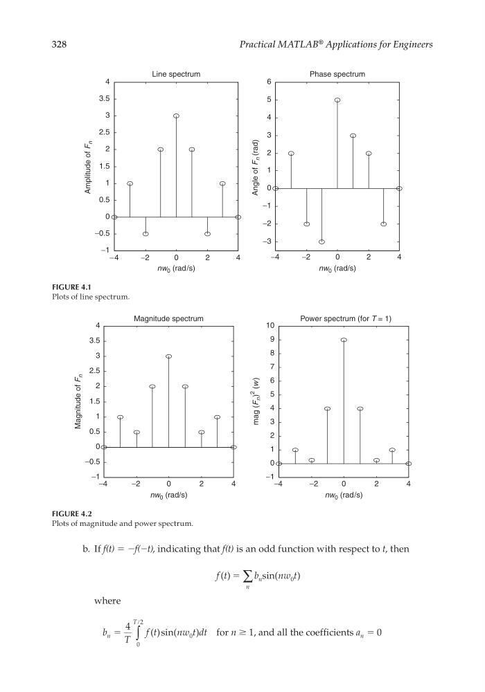
FIGURE 4.1
Plots of line spectrum.
−4
−2
0
2
4
−1
−0.5
0
0.5
1
1.5
2
2.5
3
3.5
4
nw 0 (rad/s)
Magnitude of F
n
Magnitude spectrum
−4
−2
0
2
4
−1
0
1
2
3
4
5
6
7
8
9
10
nw 0 (rad/s)
mag (F
n )
2
(w )
Power spectrum (for T = 1)
FIGURE 4.2
Plots of magnitude and power spectrum.
CRC_47760_CH004.indd 328
CRC_47760_CH004.indd 328
7/28/2008 12:25:51 PM
7/28/2008 12:25:51 PM
Practical MATLAB
® Applications for Engineers
b. If f(t) = −f(−t), indicating that f(t) is an odd function with respect to t, then
f t
b
nw t
n
( )
(
)
ϭ
sin
0
n
∑
where
b
T
f t
nw t dt
n
n
T
ϭ
4
0
0
2
( )sin(
)
ր
Ն
∫
for
1, and all the coefficients
0
a n ϭ
−4
−2
0
2
4
−1
−0.5
0
0.5
1
1.5
2
2.5
3
3.5
4
nw 0 (rad/s)
Line spectrum
−4
−2
0
2
4
−3
−2
−1
0
1
2
3
4
5
6
nw 0 (rad/s)
Angle of F
n (rad)
Phase spectrum
Amplitude of F
n
FIGURE 4.1
Plots of line spectrum.
−4
−2
0
2
4
−1
−0.5
0
0.5
1
1.5
2
2.5
3
3.5
4
nw 0 (rad/s)
Magnitude of F
n
Magnitude spectrum
−4
−2
0
2
4
−1
0
1
2
3
4
5
6
7
8
9
10
nw 0 (rad/s)
mag (F
n )
2
(w )
Power spectrum (for T = 1)
FIGURE 4.2
Plots of magnitude and power spectrum.
CRC_47760_CH004.indd 328
CRC_47760_CH004.indd 328
7/28/2008 12:25:51 PM
7/28/2008 12:25:51 PM