

Alternating Current Analysis
305
Example 3.20
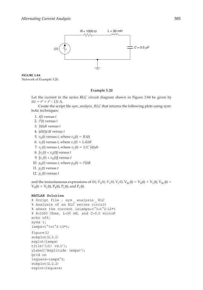
Let the current in the series RLC circuit diagram shown in Figure 3.84 be given by
i(t) = t
3
+ t
2 – 12t A.
Create the script fi le sym_analysis_RLC that returns the following plots using symbolic techniques:
1. i(t) versus t
2. i
2
(t) versus t
3. ∫i(t)dt versus t
4. (di(t))/dt versus t
5. v R (t) versus t, where v R (t) = R i(t)
6. v L (t) versus t, where v L (t) = L di/dt
7. v C (t) versus t, where v C (t) = 1/C ∫i(t)dt
8. [v L (t) + v R (t)] versus t
9. [v C (t) + v R (t)] versus t
10. p R (t) versus t, where p R (t) = i
2
(t)R
11. p L (t) versus t
12. p C (t) versus t
and the instantaneous expressions of i(t), V R (t), V L (t), V C (t), V RL (t) = V R (t) + V L (t), V RC (t) =
V R (t) + V C (t), P R (t), P L (t), and P C (t).
MATLAB Solution
% Script file : sym _ analysis _ RLC
% Analysis of an RLC series circuit
% where the current isiamps=t^3+t^2-12*t
% R=1000 Ohms, L=30 mH, and C=0.5 microF
echo off;
syms t;
iamps=t^3+t^2-12*t;
figure(1)
subplot(2,2,1)
ezplot(iamps)
title(‘i(t) vs.t’);
ylabel(‘Amplitude (amps)’);
grid on
isquare=iamps^2;
subplot(2,2,2)
ezplot(isquare)
C = 0.5 µF
L = 30 mH
i (t )
R = 1000 Ω
FIGURE 3.84
Network of Example 3.20.
CRC_47760_CH003.indd 305
CRC_47760_CH003.indd 305
7/23/2008 1:27:53 PM
7/23/2008 1:27:53 PM
305
Example 3.20
Let the current in the series RLC circuit diagram shown in Figure 3.84 be given by
i(t) = t
3
+ t
2 – 12t A.
Create the script fi le sym_analysis_RLC that returns the following plots using symbolic techniques:
1. i(t) versus t
2. i
2
(t) versus t
3. ∫i(t)dt versus t
4. (di(t))/dt versus t
5. v R (t) versus t, where v R (t) = R i(t)
6. v L (t) versus t, where v L (t) = L di/dt
7. v C (t) versus t, where v C (t) = 1/C ∫i(t)dt
8. [v L (t) + v R (t)] versus t
9. [v C (t) + v R (t)] versus t
10. p R (t) versus t, where p R (t) = i
2
(t)R
11. p L (t) versus t
12. p C (t) versus t
and the instantaneous expressions of i(t), V R (t), V L (t), V C (t), V RL (t) = V R (t) + V L (t), V RC (t) =
V R (t) + V C (t), P R (t), P L (t), and P C (t).
MATLAB Solution
% Script file : sym _ analysis _ RLC
% Analysis of an RLC series circuit
% where the current isiamps=t^3+t^2-12*t
% R=1000 Ohms, L=30 mH, and C=0.5 microF
echo off;
syms t;
iamps=t^3+t^2-12*t;
figure(1)
subplot(2,2,1)
ezplot(iamps)
title(‘i(t) vs.t’);
ylabel(‘Amplitude (amps)’);
grid on
isquare=iamps^2;
subplot(2,2,2)
ezplot(isquare)
C = 0.5 µF
L = 30 mH
i (t )
R = 1000 Ω
FIGURE 3.84
Network of Example 3.20.
CRC_47760_CH003.indd 305
CRC_47760_CH003.indd 305
7/23/2008 1:27:53 PM
7/23/2008 1:27:53 PM