

Alternating Current Analysis
301
C = 0.01 µF
V = 5 0°
L = 30 mH
R 1 = 47 kΩ
R 2 = 270 Ω
V c
I
I C
I L
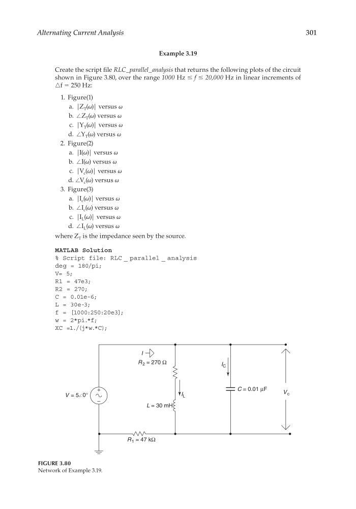
FIGURE 3.80
Network of Example 3.19.
Example 3.19
Create the script fi le RLC_parallel_analysis that returns the following plots of the circuit
shown in Figure 3.80, over the range 1000 Hz ≤ f ≤ 20,000 Hz in linear increments of
△f = 250 Hz:
1. Figure(1)
a. |Z T (ω)| versus ω
b. ∠Z T (ω) versus ω
c. |Y T (ω)| versus ω
d. ∠Y T (ω) versus ω
2. Figure(2)
a. |I(ω)| versus ω
b. ∠I(ω) versus ω
c. |V c (ω)| versus ω
d. ∠V c (ω) versus ω
3. Figure(3)
a. |I c (ω)| versus ω
b. ∠I c (ω) versus ω
c. |I L (ω)| versus ω
d. ∠I L (ω) versus ω
where Z T is the impedance seen by the source.
MATLAB Solution
% Script file: RLC _ parallel _ analysis
deg = 180/pi;
V= 5;
R1 = 47e3;
R2 = 270;
C = 0.01e-6;
L = 30e-3;
f = [1000:250:20e3];
w = 2*pi.*f;
XC =1./(j*w.*C);
CRC_47760_CH003.indd 301
CRC_47760_CH003.indd 301
7/23/2008 1:27:52 PM
7/23/2008 1:27:52 PM
301
C = 0.01 µF
V = 5 0°
L = 30 mH
R 1 = 47 kΩ
R 2 = 270 Ω
V c
I
I C
I L
FIGURE 3.80
Network of Example 3.19.
Example 3.19
Create the script fi le RLC_parallel_analysis that returns the following plots of the circuit
shown in Figure 3.80, over the range 1000 Hz ≤ f ≤ 20,000 Hz in linear increments of
△f = 250 Hz:
1. Figure(1)
a. |Z T (ω)| versus ω
b. ∠Z T (ω) versus ω
c. |Y T (ω)| versus ω
d. ∠Y T (ω) versus ω
2. Figure(2)
a. |I(ω)| versus ω
b. ∠I(ω) versus ω
c. |V c (ω)| versus ω
d. ∠V c (ω) versus ω
3. Figure(3)
a. |I c (ω)| versus ω
b. ∠I c (ω) versus ω
c. |I L (ω)| versus ω
d. ∠I L (ω) versus ω
where Z T is the impedance seen by the source.
MATLAB Solution
% Script file: RLC _ parallel _ analysis
deg = 180/pi;
V= 5;
R1 = 47e3;
R2 = 270;
C = 0.01e-6;
L = 30e-3;
f = [1000:250:20e3];
w = 2*pi.*f;
XC =1./(j*w.*C);
CRC_47760_CH003.indd 301
CRC_47760_CH003.indd 301
7/23/2008 1:27:52 PM
7/23/2008 1:27:52 PM