

Alternating Current Analysis
285
Example 3.11
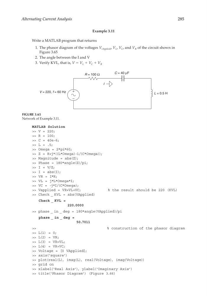
Write a MATLAB program that returns
1. The phasor diagram of the voltages V (Applied) , V L , V C , and V R of the circuit shown in
Figure 3.65
2. The angle between the I and V
3. Verify KVL, that is, V = V L + V C + V R
R = 100 Ω
I
C = 40 µF
L = 0.5 H
V = 220, f = 60 Hz
FIGURE 3.65
Network of Example 3.11.
MATLAB Solution
>> V = 220;
>> R = 100;
>> C = 40e-6;
>> L = .5;
>> Omega = 2*pi*60;
>> Z = R+j*((L*Omega)-1/(C*Omega));
>> Magnitude = abs(Z);
>> Phase = 180*angle(Z)/pi;
>> I = V/Z;
>> I = abs(I);
>> VR = I*R;
>> VL = j*L*Omega*I;
>> VC = -j*I/(C*Omega);
>> Vapplied = VR+VL+VC;
% the result should be 220 (KVL)
>> Check _ KVL = abs(VApplied)
Check _ KVL =
220.0000
>> phase _ in _ deg = 180*angle(VApplied)/pi
phase _ in _ deg =
50.7011
>>
% construction of the phasor diagram
>> L(1) = 0;
>> L(2) = VR;
>> L(3) = VR+VL;
>> L(4) = VR+VC;
>> Voltage = [0 VApplied];
>> axis(‘square’)
>> plot(real(L), imag(L), real(Voltage), imag(Voltage))
>> grid on
>> xlabel(‘Real Axis’), ylabel(‘Imaginary Axis’)
>> title(‘Phasor Diagram’) (Figure 3.66)
CRC_47760_CH003.indd 285
CRC_47760_CH003.indd 285
7/23/2008 1:27:48 PM
7/23/2008 1:27:48 PM
285
Example 3.11
Write a MATLAB program that returns
1. The phasor diagram of the voltages V (Applied) , V L , V C , and V R of the circuit shown in
Figure 3.65
2. The angle between the I and V
3. Verify KVL, that is, V = V L + V C + V R
R = 100 Ω
I
C = 40 µF
L = 0.5 H
V = 220, f = 60 Hz
FIGURE 3.65
Network of Example 3.11.
MATLAB Solution
>> V = 220;
>> R = 100;
>> C = 40e-6;
>> L = .5;
>> Omega = 2*pi*60;
>> Z = R+j*((L*Omega)-1/(C*Omega));
>> Magnitude = abs(Z);
>> Phase = 180*angle(Z)/pi;
>> I = V/Z;
>> I = abs(I);
>> VR = I*R;
>> VL = j*L*Omega*I;
>> VC = -j*I/(C*Omega);
>> Vapplied = VR+VL+VC;
% the result should be 220 (KVL)
>> Check _ KVL = abs(VApplied)
Check _ KVL =
220.0000
>> phase _ in _ deg = 180*angle(VApplied)/pi
phase _ in _ deg =
50.7011
>>
% construction of the phasor diagram
>> L(1) = 0;
>> L(2) = VR;
>> L(3) = VR+VL;
>> L(4) = VR+VC;
>> Voltage = [0 VApplied];
>> axis(‘square’)
>> plot(real(L), imag(L), real(Voltage), imag(Voltage))
>> grid on
>> xlabel(‘Real Axis’), ylabel(‘Imaginary Axis’)
>> title(‘Phasor Diagram’) (Figure 3.66)
CRC_47760_CH003.indd 285
CRC_47760_CH003.indd 285
7/23/2008 1:27:48 PM
7/23/2008 1:27:48 PM