

268
Practical MATLAB
® Applications for Engineers
C = 1e-6;
w = [200:50:2000];
XL = w*L;
XC = 1./(w*C);
plot(w,XL,’o’,w, XC,’*’)
title(‘[XL(w) and XC(w)] vs w’)
xlabel(‘frequency in rad/sec’), ylabel(‘Magnitude in Ohms’)
legend(‘XL’,’XC’)
grid on
hold; plot(w,XL,w,XC)
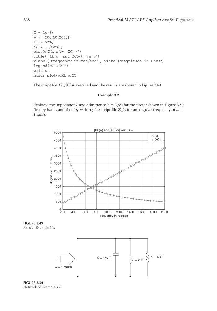
The script fi le XL_XC is executed and the results are shown in Figure 3.49.
Example 3.2
Evaluate the impedance Z and admittance Y = (1/Z) for the circuit shown in Figure 3.50
fi rst by hand, and then by writing the script fi le Z_Y, for an angular frequency of w =
1 rad/s.
FIGURE 3.49
Plots of Example 3.1.
200
400
600
800
1000 1200 1400 1600 1800 2000
0
500
1000
1500
2000
2500
3000
3500
4000
4500
5000
[XL(w) and XC(w)] versus w
frequency in rad/sec
Magnitude in Ohms
XL
XC
FIGURE 3.50
Network of Example 3.2.
R = 4 Ω
C = 1/5 F
L = 2 H
Z
w = 1 rad/s
CRC_47760_CH003.indd 268
CRC_47760_CH003.indd 268
7/23/2008 1:27:43 PM
7/23/2008 1:27:43 PM
Practical MATLAB
® Applications for Engineers
C = 1e-6;
w = [200:50:2000];
XL = w*L;
XC = 1./(w*C);
plot(w,XL,’o’,w, XC,’*’)
title(‘[XL(w) and XC(w)] vs w’)
xlabel(‘frequency in rad/sec’), ylabel(‘Magnitude in Ohms’)
legend(‘XL’,’XC’)
grid on
hold; plot(w,XL,w,XC)
The script fi le XL_XC is executed and the results are shown in Figure 3.49.
Example 3.2
Evaluate the impedance Z and admittance Y = (1/Z) for the circuit shown in Figure 3.50
fi rst by hand, and then by writing the script fi le Z_Y, for an angular frequency of w =
1 rad/s.
FIGURE 3.49
Plots of Example 3.1.
200
400
600
800
1000 1200 1400 1600 1800 2000
0
500
1000
1500
2000
2500
3000
3500
4000
4500
5000
[XL(w) and XC(w)] versus w
frequency in rad/sec
Magnitude in Ohms
XL
XC
FIGURE 3.50
Network of Example 3.2.
R = 4 Ω
C = 1/5 F
L = 2 H
Z
w = 1 rad/s
CRC_47760_CH003.indd 268
CRC_47760_CH003.indd 268
7/23/2008 1:27:43 PM
7/23/2008 1:27:43 PM