

Alternating Current Analysis
251
and
X
j C
j
j
Y
j
C
C
ϭ
ϭ
ր
ϭ
ϭ ϩ
1
1
10 3 5
1
6
6
( )( )
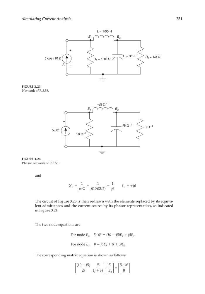
The circuit of Figure 3.23 is then redrawn with the elements replaced by its equivalent admittances and the current source by its phasor representation, as indicated
in Figure 3.24.
The two node equations are
For node E 1 , 5∠0° = (10 − j5)E 1 + j5E 2
For node E 2 , 0 = j5E 1 + (j + 3)E 2
The corresponding matrix equation is shown as follows:
(
)
(
)
10
5
5
5
3
5 0
0
1
2
Ϫ
ϩ
ϭ
Њ
j
j
j
j
E
E
⋅
∠
10 Ω
−1
+
–
5∠0°
j 6 Ω −1
3 Ω
−1
−j 5 Ω
−1
E 2
E 1
FIGURE 3.24
Phasor network of R.3.58.
R 1 = 1/10 Ω
+
–
A
5 cos (10 t )
C = 3/5 F
R 2 = 1/3 Ω
L = 1/50 H
E 2
E 1
FIGURE 3.23
Network of R.3.58.
CRC_47760_CH003.indd 251
CRC_47760_CH003.indd 251
7/23/2008 1:27:37 PM
7/23/2008 1:27:37 PM
251
and
X
j C
j
j
Y
j
C
C
ϭ
ϭ
ր
ϭ
ϭ ϩ
1
1
10 3 5
1
6
6
( )( )
The circuit of Figure 3.23 is then redrawn with the elements replaced by its equivalent admittances and the current source by its phasor representation, as indicated
in Figure 3.24.
The two node equations are
For node E 1 , 5∠0° = (10 − j5)E 1 + j5E 2
For node E 2 , 0 = j5E 1 + (j + 3)E 2
The corresponding matrix equation is shown as follows:
(
)
(
)
10
5
5
5
3
5 0
0
1
2
Ϫ
ϩ
ϭ
Њ
j
j
j
j
E
E
⋅
∠
10 Ω
−1
+
–
5∠0°
j 6 Ω −1
3 Ω
−1
−j 5 Ω
−1
E 2
E 1
FIGURE 3.24
Phasor network of R.3.58.
R 1 = 1/10 Ω
+
–
A
5 cos (10 t )
C = 3/5 F
R 2 = 1/3 Ω
L = 1/50 H
E 2
E 1
FIGURE 3.23
Network of R.3.58.
CRC_47760_CH003.indd 251
CRC_47760_CH003.indd 251
7/23/2008 1:27:37 PM
7/23/2008 1:27:37 PM