

242
Practical MATLAB
® Applications for Engineers
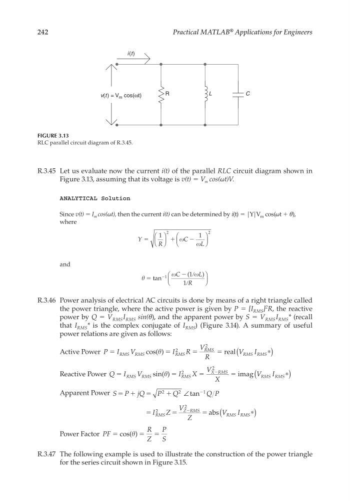
R.3.45 Let us evaluate now the current i(t) of the parallel RLC circuit diagram shown in
Figure 3.13, assuming that its voltage is v(t) = V m cos(ωt)V.
ANALYTICAL Solution
Since v(t) = I m cos(ωt), then the current i(t) can be determined by i(t) = |Y|V m cos(ωt + θ),
where
Y
R
C
L
ϭ
ϩ
Ϫ
1
1
2
2
and
ϭ
Ϫ ր
ր
Ϫ
tan
(
)
1
1
1
C
L
R
R.3.46 Power analysis of electrical AC circuits is done by means of a right triangle called
the power triangle, where the active power is given by P = [I RMS ]
2 R, the reactive
power by Q = V RMS I RMS sin(θ), and the apparent power by S = V RMS I RMS * (recall
that I RMS * is the complex conjugate of I RMS ) (Figure 3.14). A summary of useful
power relations are given as follows:
Active Power P I
V
I
R
V
R
V
I
RMS RMS
RMS
RMS
RMS RMS
ϭ
ϭ
ϭ
ϭ
cos( )
2
2
real
∗
(
)
Reactive Power Q I
V
I
X
V
X
V
I
RMS RMS
RMS
X RMS
RMS RMS
ϭ
ϭ
ϭ
ϭ
sin( )
2
2
Ϫ
imag
∗
(
)
Apparent Power S P jQ
P
Q
Q P
I
Z
V
Z
V
I
RMS
Z RMS
RMS RMS
ϭ
ϭ
ϭ
ϭ
ϭ
ϩ
ϩ
Ϫ
Ϫ
2
2
1
2
2
∠
(
)
tan
abs
∗
Power Factor PF
R
Z
P
S
ϭ
ϭ ϭ
cos( )
R.3.47 The following example is used to illustrate the construction of the power triangle
for the series circuit shown in Figure 3.15.
R
L
C
v(t ) = V m cos(ωt)
i(t)
FIGURE 3.13
RLC parallel circuit diagram of R.3.45.
CRC_47760_CH003.indd 242
CRC_47760_CH003.indd 242
7/23/2008 1:27:34 PM
7/23/2008 1:27:34 PM
Practical MATLAB
® Applications for Engineers
R.3.45 Let us evaluate now the current i(t) of the parallel RLC circuit diagram shown in
Figure 3.13, assuming that its voltage is v(t) = V m cos(ωt)V.
ANALYTICAL Solution
Since v(t) = I m cos(ωt), then the current i(t) can be determined by i(t) = |Y|V m cos(ωt + θ),
where
Y
R
C
L
ϭ
ϩ
Ϫ
1
1
2
2
and
ϭ
Ϫ ր
ր
Ϫ
tan
(
)
1
1
1
C
L
R
R.3.46 Power analysis of electrical AC circuits is done by means of a right triangle called
the power triangle, where the active power is given by P = [I RMS ]
2 R, the reactive
power by Q = V RMS I RMS sin(θ), and the apparent power by S = V RMS I RMS * (recall
that I RMS * is the complex conjugate of I RMS ) (Figure 3.14). A summary of useful
power relations are given as follows:
Active Power P I
V
I
R
V
R
V
I
RMS RMS
RMS
RMS
RMS RMS
ϭ
ϭ
ϭ
ϭ
cos( )
2
2
real
∗
(
)
Reactive Power Q I
V
I
X
V
X
V
I
RMS RMS
RMS
X RMS
RMS RMS
ϭ
ϭ
ϭ
ϭ
sin( )
2
2
Ϫ
imag
∗
(
)
Apparent Power S P jQ
P
Q
Q P
I
Z
V
Z
V
I
RMS
Z RMS
RMS RMS
ϭ
ϭ
ϭ
ϭ
ϭ
ϩ
ϩ
Ϫ
Ϫ
2
2
1
2
2
∠
(
)
tan
abs
∗
Power Factor PF
R
Z
P
S
ϭ
ϭ ϭ
cos( )
R.3.47 The following example is used to illustrate the construction of the power triangle
for the series circuit shown in Figure 3.15.
R
L
C
v(t ) = V m cos(ωt)
i(t)
FIGURE 3.13
RLC parallel circuit diagram of R.3.45.
CRC_47760_CH003.indd 242
CRC_47760_CH003.indd 242
7/23/2008 1:27:34 PM
7/23/2008 1:27:34 PM